論文用のグラフのmatplotlib template
論文用のグラフをmatplotlibで書くときのテンプレートを個人的にまとめておく。
github
- githubのjupyter notebook形式のファイルはこちら
google colaboratory
- google colaboratory で実行する場合はこちら
筆者の環境
!sw_vers
ProductName:	Mac OS X
ProductVersion:	10.14.6
BuildVersion:	18G9323
!python -V
Python 3.8.5
%matplotlib inline
%config InlineBackend.figure_format = 'png'

import time
import json

import numpy as np
import pandas as pd

import matplotlib.pyplot as plt
import matplotlib.ticker as ticker
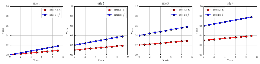
横並びに4つのグラフを描く
X = range(10)
Y = np.array(range(100)).reshape(10,10) / 100

title_list = [
  'title 1',
  'title 2',
  'title 3',
  'title 4',
]

xlabel = 'X axis'
ylabel = 'Y axis'
xlim = (0.,10.)
ylim = (0.,1.0)

plot_config_01 = {
  'marker' : '.',
  'label' :  'label A : $\sum \alpha$',
  'color' : 'r',
  'marker' : '.',
  'markersize' :12,
  'markerfacecolor' :'r',
  'markeredgewidth': 1.,
  'markeredgecolor': 'k',
}

plot_config_02 = {
  'marker' : '.',
  'label' :  'label B : $\int \beta$',
  'color' : 'b',
  'marker' : '.',
  'markersize' :12,
  'markerfacecolor' :'b',
  'markeredgewidth': 1.,
  'markeredgecolor': 'k',
}

plt.figure(figsize=(4 * 3, 3)).patch.set_facecolor('white')

plt.rcParams['font.family'] ='Times New Roman'
plt.rcParams['mathtext.fontset'] = 'stix'
plt.rcParams['xtick.direction'] = 'in'
plt.rcParams['ytick.direction'] = 'in'
plt.rcParams['xtick.major.width'] = 1.0
plt.rcParams['ytick.major.width'] = 1.0
plt.rcParams['font.size'] = 8
plt.rcParams['xtick.labelsize'] = 8
plt.rcParams['ytick.labelsize'] = 8
plt.rcParams['axes.linewidth'] = 1.0

plt.gca().yaxis.set_major_formatter(plt.FormatStrFormatter('%.2f'))
plt.gca().xaxis.get_major_formatter().set_useOffset(False)
plt.gca().yaxis.set_major_locator(ticker.MaxNLocator(integer=True))

plt.locator_params(axis='y',nbins=6)
plt.gca().yaxis.set_tick_params(which='both', direction='in',bottom=True, top=True, left=True, right=True)

for i in range(4):
  plt.subplot(1,4,i + 1)
  plt.plot(X, Y[i], **plot_config_01)
  plt.plot(X, Y[i] * 2, **plot_config_02)
  plt.grid()
  # plt.legend(loc='upper left')
  plt.legend()
  plt.xlim(xlim)
  plt.ylim(ylim)
  plt.xlabel(xlabel)
  plt.ylabel(ylabel)
  plt.title(title_list[i])
  plt.title(title_list[i])


# savefig
plt.tight_layout()

# 余白を削除
plt.savefig('./test.svg', dpi=450,  bbox_inches="tight", pad_inches=0.0)
plt.show()
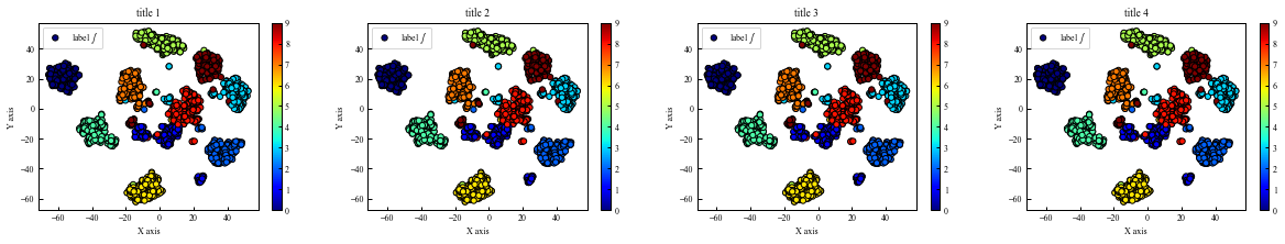
横並びに4つのtNSEのグラフを描く
from sklearn import datasets
from sklearn.manifold import TSNE

digits = datasets.load_digits()

X_reduced = TSNE(n_components=2, random_state=123).fit_transform(digits.data)
config = {
  'marker' : '.',
  'label' :  'label $\int$',
  'marker' : '.',
  's' : 112,
  'linewidths': 1.,
  'edgecolors': 'k',
  'cmap':'jet'
}

plt.figure(figsize=(4 * 3.14 + 8, 3.14)).patch.set_facecolor('white')

# plt.rcParams['font.family'] ='sans-serif'
plt.rcParams['font.family'] ='Times New Roman'
plt.rcParams['mathtext.fontset'] = 'stix'
plt.rcParams['xtick.direction'] = 'in'
plt.rcParams['ytick.direction'] = 'in'
plt.rcParams['xtick.major.width'] = 1.0
plt.rcParams['ytick.major.width'] = 1.0
plt.rcParams['font.size'] = 8
plt.rcParams['xtick.labelsize'] = 8
plt.rcParams['ytick.labelsize'] = 8
plt.rcParams['axes.linewidth'] = 1.0

plt.gca().yaxis.set_major_formatter(plt.FormatStrFormatter('%.2f'))
plt.gca().xaxis.get_major_formatter().set_useOffset(False)
plt.gca().yaxis.set_major_locator(ticker.MaxNLocator(integer=True))

plt.locator_params(axis='y',nbins=6)
plt.gca().yaxis.set_tick_params(which='both', direction='in',bottom=True, top=True, left=True, right=True)

for i in range(4):
  plt.subplot(1,4,i + 1)
  plt.scatter(X_reduced[:, 0], X_reduced[:, 1], c=digits.target, **config)
  plt.colorbar()
  plt.legend()
  plt.xlabel(xlabel)
  plt.ylabel(ylabel)
  plt.legend(loc='upper left')
  plt.title(title_list[i])


plt.savefig('./tsne.svg', dpi=450,  bbox_inches="tight", pad_inches=0.0)
plt.show()
まとめておくと便利。