Deriving the weak form of the Poisson equation for finite elements (Rewritten from an earlier blog post)
Environment
Python 3.14.6, NumPy 2.5.4, SciPy 1.18.1, SymPy 1.14.0, Matplotlib 3.11.2.
This article is a rewrite of a post from around 2013–2016, with calculations performed in the environment described above.
Overview
We multiply the Poisson equation by a test function and integrate by parts to derive its weak form. We then examine boundary conditions and assemble a matrix using one-dimensional linear elements. Python examples compare the approximate and exact solutions and show how the error decreases.
Setup
Run the code in Jupyter Notebook from top to bottom.
Imports and plotting setup
import platform
import sys
from pathlib import Path
from pprint import pprint

import matplotlib
import matplotlib.pyplot as plt
import numpy as np
import scipy
import sympy as sp
from IPython.display import Math, SVG, display
from matplotlib.ticker import FuncFormatter, NullFormatter
from scipy.sparse import coo_matrix
from scipy.sparse.linalg import spsolve

assert sys.version_info[:3] == (3, 14, 6)
assert sys.prefix != sys.base_prefix  # Check that the code is running in a virtual environment.
print("Environment: wa-src(3.14.6)")
print(f"OS: {platform.system()}, Python: {platform.python_version()}")
for module in (np, scipy, sp, matplotlib):
    print(f"{module.__name__}: {module.__version__}")

# Run from the notebook directory or the repository root.
base = Path.cwd()
if (base / "rec/cae/101/101_nb.ipynb").is_file():
    base = base / "rec/cae/101"
image_dir = base / "101_nb_files"
image_dir.mkdir(exist_ok=True)
np.set_printoptions(formatter={"float_kind": lambda x: f"{x:.2e}"})
plt.rcParams.update({"font.size": 11, "svg.fonttype": "none"})


def save_figure(fig, filename):
    """Format decimals to three significant digits and display the saved SVG."""
    for ax in fig.axes:
        for axis in (ax.xaxis, ax.yaxis):
            axis.set_major_formatter(FuncFormatter(lambda x, pos: f"{x:.2e}"))
            axis.set_minor_formatter(NullFormatter())
    fig.tight_layout()
    path = image_dir / filename
    fig.savefig(path, format="svg", bbox_inches="tight")
    plt.close(fig)
    display(SVG(filename=str(path)))
Environment: wa-src(3.14.6)
OS: Darwin, Python: 3.14.6
numpy: 2.5.4
scipy: 1.18.1
sympy: 1.14.0
matplotlib: 3.11.2
1. Strong form and boundary conditions
Consider a bounded, connected Lipschitz domain $\Omega$. Split its boundary into a Dirichlet part $\Gamma_D$ and a Neumann part $\Gamma_N$, and assume that $\Gamma_D$ has positive boundary measure. With unknown function $u$ and outward unit normal $\mathbf{n}$, the strong form is as follows.
$$ \displaystyle -\Delta u=f\ \text{in }\Omega,\qquad u=u_D\ \text{on }\Gamma_D,\qquad \nabla u\cdot\mathbf{n}=g\ \text{on }\Gamma_N. $$
Here, $f$ is the source term inside the domain, and $g$ is the normal derivative. Its sign is opposite to the normal component of the flux $-\nabla u$. The strong form requires second derivatives so that the equation holds at each point.
2. Integration by parts gives the weak form
First assume that $u$ and $v$ are sufficiently smooth. Multiply by any test function $v$ that is zero on $\Gamma_D$, and integrate over the domain.
$$ \displaystyle -\int_\Omega v\Delta u\,d\mathbf{x}=\int_\Omega fv\,d\mathbf{x}. $$
Apply the product rule and then the divergence theorem.
$$ \displaystyle \begin{aligned} \nabla\cdot(v\nabla u)&=\nabla v\cdot\nabla u+v\Delta u,\\ v\Delta u&=\nabla\cdot(v\nabla u)-\nabla v\cdot\nabla u,\\ -\int_\Omega v\Delta u\,d\mathbf{x} &=-\int_\Omega\nabla\cdot(v\nabla u)\,d\mathbf{x} +\int_\Omega\nabla v\cdot\nabla u\,d\mathbf{x}\\ &=-\int_{\partial\Omega}v\nabla u\cdot\mathbf{n}\,ds +\int_\Omega\nabla v\cdot\nabla u\,d\mathbf{x}. \end{aligned} $$
Split the boundary integral. On $\Gamma_D$, $v=0$; on $\Gamma_N$, $\nabla u\cdot\mathbf{n}=g$.
$$ \displaystyle \int_{\partial\Omega}v\nabla u\cdot\mathbf{n}\,ds =\underbrace{\int_{\Gamma_D}v\nabla u\cdot\mathbf{n}\,ds}_{0} +\int_{\Gamma_N}vg\,ds. $$
Substitute these conditions and move the boundary term to the right to obtain the weak form.
$$ \displaystyle \boxed{\int_\Omega\nabla u\cdot\nabla v\,d\mathbf{x} =\int_\Omega fv\,d\mathbf{x}+\int_{\Gamma_N}gv\,ds} $$
The Dirichlet condition constrains the functions, while the Neumann condition appears in the boundary integral on the right. Keeping the boundary term during the calculation makes its sign easier to check.
What makes the form “weak”?
$H^1(\Omega)$ is the space of square-integrable functions whose first weak derivatives are also square-integrable. Assume $f\in L^2(\Omega)$ and $g\in L^2(\Gamma_N)$, and that $u_D$ can be realized as the boundary value of an $H^1$ function.
$$ \displaystyle U=\{w\in H^1(\Omega):w|_{\Gamma_D}=u_D\},\qquad V=\{v\in H^1(\Omega):v|_{\Gamma_D}=0\}. $$
Boundary values are specified in the trace sense. The weak problem is to find $u\in U$ satisfying the equation for every $v\in V$. It requires only first derivatives, so continuous piecewise linear functions are allowed. For sufficiently smooth solutions, it corresponds to the strong form. Taking the weak form alone does not introduce an approximation.
3. Reducing the problem to finitely many unknowns
Let $u_D=0$, and let $\phi_1,\ldots,\phi_m$ be a basis of a finite-dimensional subspace $V_h$ of $V$. This is where the approximation is introduced.
$$ \displaystyle \begin{aligned} u_h&=\sum_{j=1}^m U_j\phi_j,\qquad v_h=\phi_i,\\ \int_\Omega\nabla\left(\sum_jU_j\phi_j\right)\cdot\nabla\phi_i\,d\mathbf{x} &=\int_\Omega f\phi_i\,d\mathbf{x}+\int_{\Gamma_N}g\phi_i\,ds,\\ \sum_j\underbrace{\left(\int_\Omega\nabla\phi_j\cdot\nabla\phi_i\,d\mathbf{x}\right)}_{K_{ij}}U_j &=\underbrace{\int_\Omega f\phi_i\,d\mathbf{x}+\int_{\Gamma_N}g\phi_i\,ds}_{F_i}. \end{aligned} $$
Collecting the equations for $i=1,\ldots,m$ gives a linear system with stiffness matrix $\mathbf{K}$, unknown vector $\mathbf{U}$, and load vector $\mathbf{F}$.
$$ \displaystyle \boxed{\mathbf{K}\mathbf{U}=\mathbf{F}} $$
If $u_D\ne0$, first choose a function that satisfies the boundary values. Write the solution as that function plus an unknown function that is zero on the Dirichlet boundary.
4. One-dimensional linear elements
We solve $-u^{\prime\prime}=2$ on $0\lt x\lt1$, with $u(0)=u(1)=0$. Integrate twice and apply the boundary conditions.
$$ \displaystyle u^{\prime\prime}=-2,\quad u^{\prime}=-2x+C_1,\quad u=-x^2+C_1x+C_2,\quad C_2=0,\ C_1=1,\quad u=x(1-x). $$
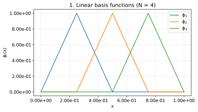
Divide the interval into $N$ equal parts, with $x_i=i/N$ and $h=1/N$. Within element $[x_e,x_{e+1}]$, set $t=x-x_e$. The local basis functions are $N_1=1-t/h$ and $N_2=t/h$.
$$ \displaystyle \begin{aligned} N_1^{\prime}&=-1/h,\quad N_2^{\prime}=1/h,\\ K^e_{11}=K^e_{22}&=\int_0^h\frac{1}{h^2}\,dt=\frac1h,\\ K^e_{12}=K^e_{21}&=\int_0^h\frac{-1}{h^2}\,dt=-\frac1h,\\ F^e_1&=\int_0^h2(1-t/h)\,dt=[2t-t^2/h]_0^h=h,\\ F^e_2&=\int_0^h2t/h\,dt=[t^2/h]_0^h=h. \end{aligned} $$
The element matrix and vector are therefore as follows. We also check the integrals with SymPy.
$$ \displaystyle \mathbf{K}^e=\frac1h\begin{bmatrix}1&-1\\-1&1\end{bmatrix},\qquad \mathbf{F}^e=h\begin{bmatrix}1\\1\end{bmatrix}. $$
t, h_symbol = sp.symbols("t h", positive=True)
shape = [1 - t / h_symbol, t / h_symbol]
ke = sp.Matrix(2, 2, lambda i, j: sp.integrate(
    sp.diff(shape[i], t) * sp.diff(shape[j], t), (t, 0, h_symbol)
))
fe = sp.Matrix([sp.integrate(2 * n, (t, 0, h_symbol)) for n in shape])
assert ke == sp.Matrix([[1, -1], [-1, 1]]) / h_symbol
assert fe == sp.Matrix([h_symbol, h_symbol])
display(Math(r"\mathbf{K}^e=" + sp.latex(ke)))
display(Math(r"\mathbf{F}^e=" + sp.latex(fe)))

# Each global hat basis function spans two neighboring elements.
grid = np.linspace(0, 1, 401)
fig, ax = plt.subplots(figsize=(7, 4))
for i in range(1, 4):
    phi = np.maximum(1 - np.abs(grid - i / 4) / (1 / 4), 0)
    ax.plot(grid, phi, label=rf"$\phi_{i}$")
ax.set(xlabel="$x$", ylabel=r"$\phi_i(x)$", title="1. Linear basis functions (N = 4)")
ax.legend()
ax.grid(alpha=0.300)
save_figure(fig, "01_basis.svg")
$$ \displaystyle \mathbf{K}^e=\left[\begin{matrix}\frac{1}{h} & - \frac{1}{h}\\- \frac{1}{h} & \frac{1}{h}\end{matrix}\right] $$
$$ \displaystyle \mathbf{F}^e=\left[\begin{matrix}h\\h\end{matrix}\right] $$
Assembly and elimination of boundary values
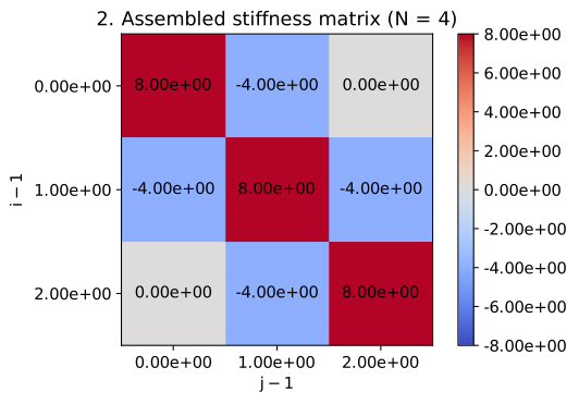
Add contributions at shared nodes. At an interior node, the diagonal entry is $2/h$, the neighboring entries are $-1/h$, and the load is $2h$. Removing the known zero endpoint values leaves $N-1$ unknowns. The following implementation is specific to this problem. A different right-hand side also requires different element load integrals.
def solve_poisson(n):
    """Solve -u'' = 2 with zero endpoint values using linear elements on a uniform mesh."""
    nodes = np.linspace(0, 1, n + 1)
    h = 1 / n
    local_k = np.array([[1, -1], [-1, 1]]) / h
    rows, cols, values = [], [], []
    load = np.zeros(n + 1)
    for e in range(n):
        ids = [e, e + 1]
        load[ids] += h  # Each local nodal load is h.
        for a in range(2):
            for b in range(2):
                rows.append(ids[a])
                cols.append(ids[b])
                values.append(local_k[a, b])
    # Conversion to CSR sums contributions for the same node pair.
    stiffness = coo_matrix((values, (rows, cols)), shape=(n + 1, n + 1)).tocsr()
    interior_k = stiffness[1:-1, 1:-1]
    interior_f = load[1:-1]
    solution = np.zeros(n + 1)
    solution[1:-1] = spsolve(interior_k, interior_f)
    return nodes, solution, interior_k, interior_f


nodes, solution, stiffness, load = solve_poisson(4)
pprint({"K": stiffness.toarray(), "F": load, "U": solution[1:-1]}, sort_dicts=False)
residual = np.linalg.norm(stiffness @ solution[1:-1] - load)
pprint({"residual_norm": f"{residual:.2e}"})

fig, ax = plt.subplots(figsize=(6, 4))
mesh = ax.imshow(stiffness.toarray(), cmap="coolwarm", vmin=-8, vmax=8)
ax.set(xticks=range(3), yticks=range(3), xlabel="$j-1$", ylabel="$i-1$",
       title="2. Assembled stiffness matrix (N = 4)")
for (i, j), value in np.ndenumerate(stiffness.toarray()):
    ax.text(j, i, f"{value:.2e}", ha="center", va="center")
fig.colorbar(mesh, ax=ax)
save_figure(fig, "02_stiffness.svg")
{'K': array([[8.00e+00, -4.00e+00, 0.00e+00],
       [-4.00e+00, 8.00e+00, -4.00e+00],
       [0.00e+00, -4.00e+00, 8.00e+00]]),
 'F': array([5.00e-01, 5.00e-01, 5.00e-01]),
 'U': array([1.88e-01, 2.50e-01, 1.87e-01])}
{'residual_norm': '1.92e-16'}
5. Checking the solution and its error
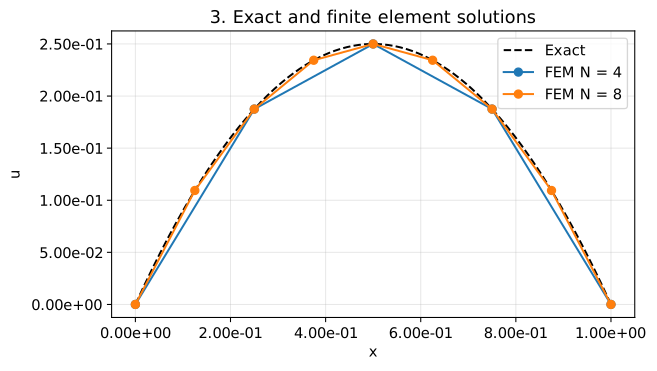
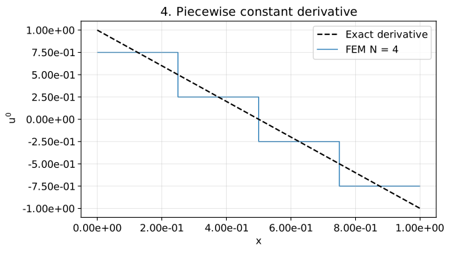
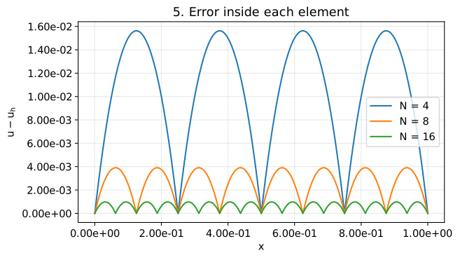
In this example, the nodal values agree with the exact solution, but the straight segments still have error between nodes. The derivative is constant on each element. Comparing nodal values alone therefore does not measure accuracy inside the elements.
exact = grid * (1 - grid)
fig, ax = plt.subplots(figsize=(7, 4))
ax.plot(grid, exact, "k--", label="Exact")
for n in (4, 8):
    x, u, _, _ = solve_poisson(n)
    ax.plot(x, u, "o-", label=f"FEM N = {n}")
ax.set(xlabel="$x$", ylabel="$u$", title="3. Exact and finite element solutions")
ax.legend()
ax.grid(alpha=0.300)
save_figure(fig, "03_solution.svg")

fig, ax = plt.subplots(figsize=(7, 4))
ax.plot(grid, 1 - 2 * grid, "k--", label="Exact derivative")
ax.stairs(np.diff(solution) / np.diff(nodes), nodes, baseline=None, label="FEM N = 4")
ax.set(xlabel="$x$", ylabel="$u'$", title="4. Piecewise constant derivative")
ax.legend()
ax.grid(alpha=0.300)
save_figure(fig, "04_derivative.svg")

fig, ax = plt.subplots(figsize=(7, 4))
for n in (4, 8, 16):
    x, u, _, _ = solve_poisson(n)
    ax.plot(grid, exact - np.interp(grid, x, u), label=f"N = {n}")
ax.set(xlabel="$x$", ylabel="$u-u_h$", title="5. Error inside each element")
ax.legend()
ax.grid(alpha=0.300)
save_figure(fig, "05_error.svg")
Error size and convergence order
Nodal agreement follows by substituting $U_i=x_i(1-x_i)$ into the interior equation $(-U_{i-1}+2U_i-U_{i+1})/h=2h$. Inside an element, the error $e=u-u_h$ is zero at both ends and satisfies $e^{\prime\prime}=-2$, so $e=t(h-t)$.
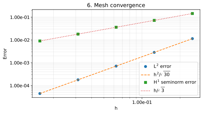
$$ \displaystyle \begin{aligned} \|e\|_{L^2}^2 &=N\int_0^h t^2(h-t)^2dt =N[h^2t^3/3-ht^4/2+t^5/5]_0^h\\ &=Nh^5(1/3-1/2+1/5)=h^4/30,\\ |e|_{H^1}^2 &=N\int_0^h(h-2t)^2dt =N[h^2t-2ht^2+4t^3/3]_0^h=h^2/3. \end{aligned} $$
We used $Nh=1$. Thus $\|e\|_{L^2}=h^2/\sqrt{30}$ and $|e|_{H^1}=h/\sqrt3$. The second quantity measures derivative error and is called the $H^1$ seminorm. We use three-point Gauss quadrature. The squared error is a fourth-degree polynomial in this example, so the rule integrates it exactly apart from rounding error.
def error_norms(nodes, solution):
    """Integrate solution and derivative errors element by element."""
    q, weights = np.polynomial.legendre.leggauss(3)
    l2_sq, h1_sq = 0, 0
    for e, h in enumerate(np.diff(nodes)):
        fraction = (q + 1) / 2
        xq = nodes[e] + h * fraction
        uh = (1 - fraction) * solution[e] + fraction * solution[e + 1]
        duh = (solution[e + 1] - solution[e]) / h
        l2_sq += h / 2 * np.dot(weights, (xq * (1 - xq) - uh) ** 2)
        h1_sq += h / 2 * np.dot(weights, (1 - 2 * xq - duh) ** 2)
    return np.sqrt(l2_sq), np.sqrt(h1_sq)


counts = np.array([4, 8, 16, 32, 64])
hs = 1 / counts
errors = np.array([error_norms(*solve_poisson(int(n))[:2]) for n in counts])
orders = np.log(errors[:-1] / errors[1:]) / np.log(2)
table = []
for i, n in enumerate(counts):
    table.append({"N": int(n), "L2": f"{errors[i, 0]:.2e}",
                  "H1_semi": f"{errors[i, 1]:.2e}",
                  "p_L2": "-" if i == 0 else f"{orders[i-1, 0]:.2e}",
                  "p_H1": "-" if i == 0 else f"{orders[i-1, 1]:.2e}"})
pprint(table, sort_dicts=False)

# Check the analytic formulas to detect assembly or integration errors.
np.testing.assert_allclose(errors[:, 0], hs**2 / np.sqrt(30), rtol=1.00e-8)
np.testing.assert_allclose(errors[:, 1], hs / np.sqrt(3), rtol=1.00e-8)
print("Confirmed agreement between analytic formulas and numerical integration.")

fig, ax = plt.subplots(figsize=(7, 4))
ax.loglog(hs, errors[:, 0], "o", label=r"$L^2$ error")
ax.loglog(hs, hs**2 / np.sqrt(30), "--", label=r"$h^2/\sqrt{30}$")
ax.loglog(hs, errors[:, 1], "s", label=r"$H^1$ seminorm error")
ax.loglog(hs, hs / np.sqrt(3), ":", label=r"$h/\sqrt{3}$")
ax.set(xlabel="$h$", ylabel="Error", title="6. Mesh convergence")
ax.legend()
ax.grid(which="both", alpha=0.300)
save_figure(fig, "06_convergence.svg")
[{'N': 4, 'L2': '1.14e-02', 'H1_semi': '1.44e-01', 'p_L2': '-', 'p_H1': '-'},
 {'N': 8,
  'L2': '2.85e-03',
  'H1_semi': '7.22e-02',
  'p_L2': '2.00e+00',
  'p_H1': '1.00e+00'},
 {'N': 16,
  'L2': '7.13e-04',
  'H1_semi': '3.61e-02',
  'p_L2': '2.00e+00',
  'p_H1': '1.00e+00'},
 {'N': 32,
  'L2': '1.78e-04',
  'H1_semi': '1.80e-02',
  'p_L2': '2.00e+00',
  'p_H1': '1.00e+00'},
 {'N': 64,
  'L2': '4.46e-05',
  'H1_semi': '9.02e-03',
  'p_L2': '2.00e+00',
  'p_H1': '1.00e+00'}]
Confirmed agreement between analytic formulas and numerical integration.
Conclusion
We derived the weak form of the Poisson equation by integration by parts, then checked discretization with linear elements and the resulting error.
Moving a derivative onto the test function reduces the required derivatives of the solution from second to first order. Boundary conditions enter through the function spaces and the boundary integral. Choosing a finite-dimensional basis gives a linear system. In this example, halving the mesh width reduced the $L^2$ error to $1/4$ and the derivative error to $1/2$.