How the Galerkin method leads to finite elements (Rewritten from an earlier blog post)
Environment
Python 3.14.6, NumPy 2.5.4, SciPy 1.18.1, SymPy 1.14.0, Matplotlib 3.11.2.
This article is a rewrite of a post from around 2013–2016, with calculations performed in the environment described above.
Overview
The Galerkin method uses the same finite-dimensional space for the approximate solution and test functions. Dividing the domain into elements and choosing local piecewise polynomial basis functions gives the standard Galerkin finite element method. We use a one-dimensional Poisson equation to work through the weak form and element assembly, then check the approximate solution and errors in Python.
Setup
Run the code in Jupyter Notebook from top to bottom.
Imports and plotting setup
import platform
import sys
from pathlib import Path
from pprint import pprint

import matplotlib
import matplotlib.pyplot as plt
import numpy as np
import scipy
import sympy as sp
from IPython.display import Latex, display
from matplotlib.ticker import FuncFormatter, NullFormatter
from scipy.sparse import lil_matrix
from scipy.sparse.linalg import spsolve

%matplotlib inline
%config InlineBackend.figure_format = 'svg'

assert sys.version_info[:3] == (3, 14, 6), 'Select wa-src(3.14.6)'
print('Environment: wa-src(3.14.6)')
print('Python:', platform.python_version())
print('OS:', platform.system(), platform.release())
for name, module in [('NumPy', np), ('SciPy', scipy),
                     ('SymPy', sp), ('Matplotlib', matplotlib)]:
    print(f'{name}: {module.__version__}')

# Save beside the notebook; also support running from the repository root.
workdir = Path.cwd()
article_dir = workdir / 'rec' / 'cae' / '102'
output_dir = (article_dir if article_dir.is_dir() else workdir) / '102_nb_files'
output_dir.mkdir(exist_ok=True)

def sig(value):
    """Show three significant digits, retaining trailing zeros."""
    # Adjust tiny floating-point artifacts and round to three digits for display only.
    return f'{float(f"{float(value):.14g}"):#.3g}'

np.set_printoptions(formatter={'float_kind': sig})
plt.rcParams.update({'font.size': 11, 'svg.fonttype': 'none'})

def save_figure(fig, filename):
    """Format axis values, save the SVG, and display it in the notebook."""
    for ax in fig.axes:
        for axis in (ax.xaxis, ax.yaxis):
            axis.set_major_formatter(FuncFormatter(lambda value, pos: sig(value)))
            axis.set_minor_formatter(NullFormatter())
    fig.savefig(output_dir / filename, format='svg', bbox_inches='tight')
    plt.show()
    plt.close(fig)
Environment: wa-src(3.14.6)
Python: 3.14.6
OS: Darwin 25.5.0
NumPy: 2.5.4
SciPy: 1.18.1
SymPy: 1.14.0
Matplotlib: 3.11.2
1. Putting the differential equation in weak form
We consider a problem with fixed values at both ends.
$$ \displaystyle -u^{\prime\prime}(x)=2\quad(0\lt x\lt1),\qquad u(0)=u(1)=0. $$
Integration gives $u^{\prime}=-2x+C_1$ and $u=-x^2+C_1x+C_2$. The boundary conditions give $C_2=0$ and $C_1=1$, so the exact solution is $u=x(1-x)$.
Multiply by a test function $v$ that is zero at both ends, and integrate by parts.
$$ \displaystyle \begin{aligned} \int_0^1(-u^{\prime\prime})v\,dx&=\int_0^1 2v\,dx,\\ -[u^{\prime}v]_0^1+\int_0^1u^{\prime}v^{\prime}\,dx&=\int_0^1 2v\,dx,\\ \int_0^1u^{\prime}v^{\prime}\,dx&=\int_0^1 2v\,dx. \end{aligned} $$
The last equation is the weak form. Let $V=H_0^1(0,1)$ be the space of functions with square-integrable values and weak first derivatives, and zero endpoint values. We seek $u\in V$ satisfying the equation for every $v\in V$. Second derivatives are no longer required, so piecewise linear approximations with slope changes at nodes are allowed.
2. Using Galerkin’s method to obtain finitely many unknowns
Choose $V_h=\operatorname{span}\{\phi_1,\ldots,\phi_{n-1}\}\subset V$ and expand the approximate solution. Choosing test functions from the same $V_h$ is the Galerkin condition.
$$ \displaystyle \begin{aligned} u_h&=\sum_{j=1}^{n-1}U_j\phi_j,\\ \int_0^1\left(\sum_j U_j\phi_j^{\prime}\right)\phi_i^{\prime}\,dx &=\int_0^1 2\phi_i\,dx,\\ \sum_j\underbrace{\left(\int_0^1\phi_i^{\prime}\phi_j^{\prime}\,dx\right)}_{K_{ij}}U_j &=\underbrace{\int_0^1 2\phi_i\,dx}_{F_i},\\ \mathbf{K}\mathbf{U}&=\mathbf{F}. \end{aligned} $$
Subtracting the weak forms for the exact and approximate solutions gives $\int_0^1(u-u_h)^{\prime}v_h^{\prime}\,dx=0$. This is Galerkin orthogonality. It does not mean that the error is zero at every point.
3. Local basis functions lead to finite elements
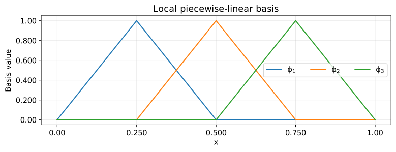
Divide the interval into $n$ equal parts, with $h=1/n$ and $x_i=ih$. Use a basis function that is one at interior node $i$ and zero at all other nodes.
$$ \displaystyle \phi_i(x)=\begin{cases} (x-x_{i-1})/h&x_{i-1}\le x\le x_i,\\ (x_{i+1}-x)/h&x_i\lt x\le x_{i+1},\\ 0&\text{otherwise}. \end{cases} $$
Since $\phi_i(x_j)=\delta_{ij}$, we have $u_h(x_i)=U_i$. Distinct basis functions overlap only for neighboring nodes, so $K_{ij}=0$ when $|i-j|\gt 1$. The elements, local basis functions, and node connections define this linear finite element space.
The Galerkin method itself does not restrict the basis. Trigonometric functions extending across the whole domain are also possible. Finite elements arise here because we join elementwise polynomials as well as use a weak form. Comparing basis overlap with the nonzero matrix entries shows why a local basis produces a sparse matrix.
# Plot the interior basis for four elements; endpoint degrees of freedom are fixed.
n = 4
nodes = np.linspace(0, 1, n + 1)
grid = np.linspace(0, 1, 801)
h = 1 / n

fig, ax = plt.subplots(figsize=(8, 3), layout='constrained')
for i in range(1, n):
    phi = np.maximum(1 - np.abs(grid - nodes[i]) / h, 0)
    ax.plot(grid, phi, label=rf'$\phi_{i}$')
ax.set(xlabel='$x$', ylabel='Basis value', title='Local piecewise-linear basis')
ax.set_xticks(nodes)
ax.legend(ncol=3)
ax.grid(alpha=0.250)
save_figure(fig, '01_basis.svg')
4. Integrating the element matrix
Take one element $[a,a+h]$ and set $s=x-a$. The local shape functions are $N_1=1-s/h$ and $N_2=s/h$, with derivatives $N_1^{\prime}=-1/h$ and $N_2^{\prime}=1/h$.
$$ \displaystyle \begin{aligned} K_{11}^{(e)}=K_{22}^{(e)}&=\int_0^h\frac{1}{h^2}\,ds=\frac{1}{h},\\ K_{12}^{(e)}=K_{21}^{(e)}&=\int_0^h\frac{-1}{h^2}\,ds=-\frac{1}{h},\\ F_1^{(e)}&=2\int_0^h(1-s/h)\,ds=2[h-h/2]=h,\\ F_2^{(e)}&=2\int_0^h s/h\,ds=2[h/2]=h,\\ \mathbf{K}^{(e)}&=\frac{1}{h}\begin{bmatrix}1&-1\\-1&1\end{bmatrix}, \quad\mathbf{F}^{(e)}=h\begin{bmatrix}1\\1\end{bmatrix}. \end{aligned} $$
We also integrate with SymPy and show the formulas using display().
s, he = sp.symbols('s h', positive=True)
shape = sp.Matrix([1 - s / he, s / he])
derivative = shape.diff(s)
element_k = sp.integrate(derivative * derivative.T, (s, 0, he))
element_f = sp.integrate(2 * shape, (s, 0, he))

display(Latex(r'$$\displaystyle \mathbf{K}^{(e)}=' + sp.latex(element_k) + r'$$'))
display(Latex(r'$$\displaystyle \mathbf{F}^{(e)}=' + sp.latex(element_f) + r'$$'))
$$ \displaystyle \mathbf{K}^{(e)}=\left[\begin{matrix}\frac{1}{h} & - \frac{1}{h}\\- \frac{1}{h} & \frac{1}{h}\end{matrix}\right] $$
$$ \displaystyle \mathbf{F}^{(e)}=\left[\begin{matrix}h\\h\end{matrix}\right] $$
5. Assembling and solving the global system
Map local indices $(1,2)$ of element $e$ to global nodes $(e,e+1)$, and add the shared contributions. Two elements meet at each interior node, giving $K_{ii}=2/h$, $K_{i,i\pm1}=-1/h$, and $F_i=2h$. With $n=4$, removing the known endpoint values gives this system.
$$ \displaystyle \begin{bmatrix}8&-4&0\\-4&8&-4\\0&-4&8\end{bmatrix} \begin{bmatrix}U_1\\U_2\\U_3\end{bmatrix} =\begin{bmatrix}1/2\\1/2\\1/2\end{bmatrix}. $$
Subtracting the third equation from the first gives $U_1=U_3$. The second gives $U_2=U_1+1/16$. Substitution into the first gives $4U_1-1/4=1/2$, hence $U_1=U_3=3/16$ and $U_2=1/4$.
def solve_fem(n):
    """Solve -u''=2 with zero endpoint values using linear elements on a uniform mesh."""
    nodes = np.linspace(0, 1, n + 1)
    stiffness = lil_matrix((n + 1, n + 1), dtype=float)
    load = np.zeros(n + 1)

    for e in range(n):
        length = nodes[e + 1] - nodes[e]
        local_k = np.array([[1, -1], [-1, 1]]) / length
        local_f = length * np.ones(2)
        indices = [e, e + 1]

        # Add contributions at shared nodes instead of overwriting them.
        for a, i in enumerate(indices):
            load[i] += local_f[a]
            for b, j in enumerate(indices):
                stiffness[i, j] += local_k[a, b]

    # Zero boundary values let us keep only the interior entries.
    interior_k = stiffness.tocsr()[1:-1, 1:-1]
    interior_f = load[1:-1]
    values = np.zeros(n + 1)
    values[1:-1] = spsolve(interior_k, interior_f)
    return nodes, values, interior_k, interior_f

nodes, values, stiffness, load = solve_fem(4)
print('Interior stiffness matrix, load vector, and solution at all nodes:')
pprint(stiffness.toarray())
pprint(load)
pprint(values)

# Check the hand-computed solution and the discrete equations.
np.testing.assert_allclose(values, [0, 3 / 16, 1 / 4, 3 / 16, 0], atol=1e-14)
np.testing.assert_allclose(stiffness @ values[1:-1], load, atol=1e-14)
residual = stiffness @ values[1:-1] - load
pprint({'maximum absolute discrete residual': sig(np.max(np.abs(residual)))})

fig, ax = plt.subplots(figsize=(5, 4), layout='constrained')
_, _, matrix16, _ = solve_fem(16)
ax.spy(matrix16, markersize=7)
ax.set(xlabel='Column index', ylabel='Row index', title='Nonzero entries: 16 elements')
ax.set_xticks([0, 7, 14])
ax.set_yticks([0, 7, 14])
save_figure(fig, '02_sparsity.svg')
Interior stiffness matrix, load vector, and solution at all nodes:
array([[8.00, -4.00, 0.00],
       [-4.00, 8.00, -4.00],
       [0.00, -4.00, 8.00]])
array([0.500, 0.500, 0.500])
array([0.00, 0.188, 0.250, 0.188, 0.00])
{'maximum absolute discrete residual': '1.11e-16'}
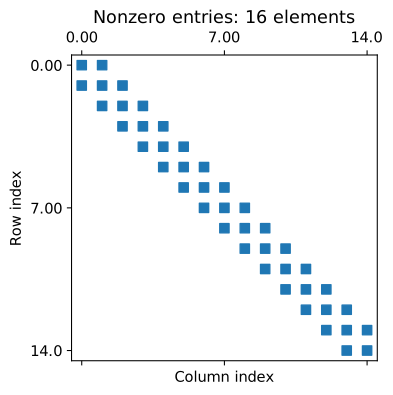
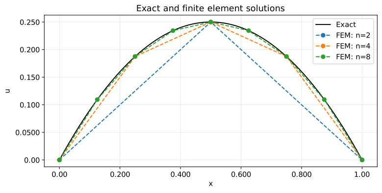
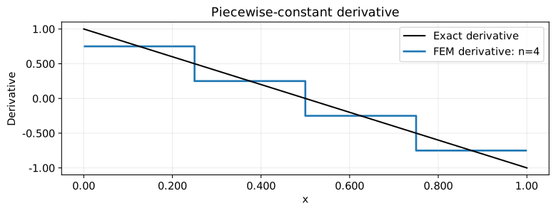
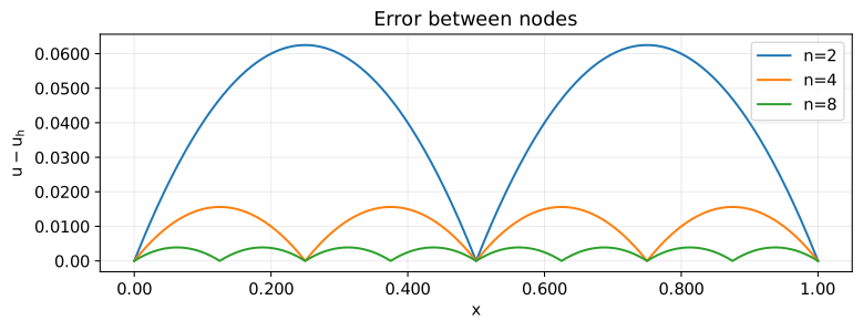
The nodal values match the exact solution here, but error remains between nodes. Such nodal agreement does not hold for every equation. The figures show the solution, derivative, and error in that order. Evaluating the piecewise linear second derivative only inside elements misses the slope jumps at nodes, so it does not correctly test the residual of the original differential equation.
def exact(x):
    return x * (1 - x)

grid = np.linspace(0, 1, 1001)
fig, ax = plt.subplots(figsize=(8, 4), layout='constrained')
ax.plot(grid, exact(grid), color='black', label='Exact')
for n in (2, 4, 8):
    nodes, values, _, _ = solve_fem(n)
    ax.plot(nodes, values, 'o--', label=f'FEM: n={n}')
ax.set(xlabel='$x$', ylabel='$u$', title='Exact and finite element solutions')
ax.legend()
ax.grid(alpha=0.250)
save_figure(fig, '03_solution.svg')

nodes, values, _, _ = solve_fem(4)
slopes = np.diff(values) / np.diff(nodes)
fig, ax = plt.subplots(figsize=(8, 3), layout='constrained')
ax.plot(grid, 1 - 2 * grid, color='black', label="Exact derivative")
ax.stairs(slopes, nodes, baseline=None, label='FEM derivative: n=4', linewidth=2)
ax.set(xlabel='$x$', ylabel="Derivative", title='Piecewise-constant derivative')
ax.legend()
ax.grid(alpha=0.250)
save_figure(fig, '04_derivative.svg')

fig, ax = plt.subplots(figsize=(8, 3), layout='constrained')
for n in (2, 4, 8):
    nodes, values, _, _ = solve_fem(n)
    error = exact(grid) - np.interp(grid, nodes, values)
    ax.plot(grid, error, label=f'n={n}')
ax.set(xlabel='$x$', ylabel='$u-u_h$', title='Error between nodes')
ax.legend()
ax.grid(alpha=0.250)
save_figure(fig, '05_error.svg')
6. Error under mesh refinement
The interior equation is $2U_i-U_{i-1}-U_{i+1}=2h^2$. Substituting $U_i=x_i(1-x_i)$ makes the left side $2h^2$ and also satisfies the boundary conditions. Thus $u_h$ is the piecewise linear interpolant of the exact nodal values.
Let $s$ be the distance from an element’s left endpoint. Then $u(a+s)=u(a)+(1-2a)s-s^2$ and $u_h(a+s)=u(a)+(1-2a-h)s$. The error is $e=s(h-s)$, and its derivative is $e^{\prime}=h-2s$.
$$ \displaystyle \begin{aligned} \|e\|_{L^2}^2 &=n\int_0^h(h^2s^2-2hs^3+s^4)\,ds\\ &=n(h^5/3-h^5/2+h^5/5)=h^4/30,\\ |e|_{H^1}^2 &=n\int_0^h(h^2-4hs+4s^2)\,ds\\ &=n(h^3-2h^3+4h^3/3)=h^2/3. \end{aligned} $$
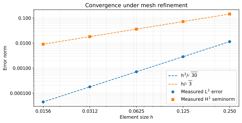
Therefore $\|e\|_{L^2}=h^2/\sqrt{30}$ and $|e|_{H^1}=h/\sqrt{3}$. The latter is a seminorm measuring derivative error. We use three-point Gauss quadrature on each element. The squared errors have degree at most four, so the integrals are exact apart from rounding error.
def measure_errors(nodes, values):
    """Integrate each element separately to avoid crossing derivative jumps at nodes."""
    points, weights = np.polynomial.legendre.leggauss(3)
    l2_squared = 0
    h1_squared = 0
    for i, length in enumerate(np.diff(nodes)):
        # Map quadrature nodes from [-1, 1] to the element.
        t = (points + 1) / 2
        xq = nodes[i] + length * t
        uq = (1 - t) * values[i] + t * values[i + 1]
        slope = (values[i + 1] - values[i]) / length
        l2_squared += length / 2 * np.dot(weights, (exact(xq) - uq) ** 2)
        h1_squared += length / 2 * np.dot(weights, (1 - 2 * xq - slope) ** 2)
    return np.sqrt(l2_squared), np.sqrt(h1_squared)

counts = np.array([4, 8, 16, 32, 64])
sizes = 1 / counts
errors = np.array([measure_errors(*solve_fem(int(n))[:2]) for n in counts])
theory_l2 = sizes ** 2 / np.sqrt(30)
theory_h1 = sizes / np.sqrt(3)
np.testing.assert_allclose(errors[:, 0], theory_l2, rtol=1e-10)
np.testing.assert_allclose(errors[:, 1], theory_h1, rtol=1e-10)

# Compute the observed order as p = log(E_h / E_{h/2}) / log(2).
rates = np.log(errors[:-1] / errors[1:]) / np.log(2)
rows = []
for i, n in enumerate(counts):
    rows.append({'n': int(n), 'h': sig(sizes[i]),
                 'L2': sig(errors[i, 0]), 'H1 seminorm': sig(errors[i, 1]),
                 'p(L2)': '-' if i == 0 else sig(rates[i - 1, 0]),
                 'p(H1)': '-' if i == 0 else sig(rates[i - 1, 1])})
pprint(rows, sort_dicts=False)

fig, ax = plt.subplots(figsize=(8, 4), layout='constrained')
ax.loglog(sizes, theory_l2, '--', color='C0', label=r'$h^2/\sqrt{30}$')
ax.loglog(sizes, theory_h1, '--', color='C1', label=r'$h/\sqrt{3}$')
ax.loglog(sizes, errors[:, 0], 'o', color='C0', label=r'Measured $L^2$ error')
ax.loglog(sizes, errors[:, 1], 's', color='C1', label=r'Measured $H^1$ seminorm')
ax.set(xlabel='Element size $h$', ylabel='Error norm', title='Convergence under mesh refinement')
ax.set_xticks(sizes)
ax.legend()
ax.grid(which='both', alpha=0.250)
save_figure(fig, '06_convergence.svg')
[{'n': 4,
  'h': '0.250',
  'L2': '0.0114',
  'H1 seminorm': '0.144',
  'p(L2)': '-',
  'p(H1)': '-'},
 {'n': 8,
  'h': '0.125',
  'L2': '0.00285',
  'H1 seminorm': '0.0722',
  'p(L2)': '2.00',
  'p(H1)': '1.00'},
 {'n': 16,
  'h': '0.0625',
  'L2': '0.000713',
  'H1 seminorm': '0.0361',
  'p(L2)': '2.00',
  'p(H1)': '1.00'},
 {'n': 32,
  'h': '0.0312',
  'L2': '0.000178',
  'H1 seminorm': '0.0180',
  'p(L2)': '2.00',
  'p(H1)': '1.00'},
 {'n': 64,
  'h': '0.0156',
  'L2': '4.46e-05',
  'H1 seminorm': '0.00902',
  'p(L2)': '2.00',
  'p(H1)': '1.00'}]
Conclusion
Applying Galerkin’s method to the weak form and choosing local piecewise polynomial basis functions gives the finite element method used here.
The weak form reduces the derivatives required of the solution from second to first order. The local basis allows sparse matrices and elementwise calculations. With these linear elements, the $L^2$ solution error is proportional to $h^2$ and the derivative error to $h$. These results apply to the problem studied here, with a uniform mesh and a smooth exact solution.