Why does Newton’s method converge quadratically? (Rewritten from an earlier blog post)
Environment
Python 3.14.6, NumPy 2.5.4, SymPy 1.14.0, Matplotlib 3.11.2 (Jupyter Notebook).
This article is a rewrite of a post from around 2013–2016, with calculations performed in the environment described above.
Overview
Newton’s method is an iterative method that takes the $x$ coordinate where a tangent line meets the horizontal axis as the next approximation. If the function is twice continuously differentiable and the iteration starts close enough to a simple root, the first-order error term cancels, giving at least quadratic convergence.
We derive the error relation using a Taylor expansion and check it by computing the positive solution of $x^2-2=0$. We also examine slower convergence at multiple roots, examples that fail to converge from some starting points, and the accuracy limit caused by rounding errors.
Setup
Run the code in Jupyter Notebook from top to bottom. Round numbers to three significant digits only when displaying them.
import platform
from decimal import Decimal, getcontext
from importlib.metadata import version
from pathlib import Path
from pprint import pprint

import matplotlib.pyplot as plt
import numpy as np
import sympy as sp
from IPython.display import Math, display
from matplotlib.ticker import FuncFormatter, MaxNLocator
from matplotlib_inline.backend_inline import set_matplotlib_formats

%matplotlib inline
set_matplotlib_formats("svg")

print("Python:", platform.python_version())
pprint({name: version(name) for name in ("numpy", "matplotlib", "sympy")})

# Use 120-digit decimal arithmetic to evaluate errors. Convert only plotting arrays to float.
getcontext().prec = 120
np.set_printoptions(formatter={"float_kind": lambda value: f"{value:.2e}"})
figure_dir = Path("101_nb_files")
figure_dir.mkdir(exist_ok=True)
plt.rcParams.update({"font.size": 11, "svg.fonttype": "none"})


def tick_label(value, position):
    """Keep integers as they are; display decimals with three significant digits, including trailing zeros."""
    if float(value).is_integer() and abs(value) < 1000:
        return str(int(value))
    return f"{value:#.3g}"


def save_figure(fig, name):
    """Format the axes, save the figure as SVG, and display it in the output area."""
    for ax in fig.axes:
        if ax.get_xscale() == "linear":
            ax.xaxis.set_major_formatter(FuncFormatter(tick_label))
        if ax.get_yscale() == "linear":
            ax.yaxis.set_major_formatter(FuncFormatter(tick_label))
        ax.grid(True, alpha=0.250)
    fig.tight_layout()
    fig.savefig(figure_dir / name, format="svg", bbox_inches="tight")
    plt.show()
    plt.close(fig)
Python: 3.14.6
{'matplotlib': '3.11.2', 'numpy': '2.5.4', 'sympy': '1.14.0'}
1. Deriving the update from a tangent line
Let $\alpha$ be a solution of $f(x)=0$, and let $x_n$ be an approximation. Write the tangent line at $(x_n,f(x_n))$ as $y=q_n(x)$. If $f^{\prime}(x_n)\ne0$, its intersection with the horizontal axis has the following $x$ coordinate.
$$ \displaystyle \begin{gathered} q_n(x)=f(x_n)+f^{\prime}(x_n)(x-x_n),\\ 0=f(x_n)+f^{\prime}(x_n)(x_{n+1}-x_n),\\ x_{n+1}-x_n=-\frac{f(x_n)}{f^{\prime}(x_n)},\\ x_{n+1}=x_n-\frac{f(x_n)}{f^{\prime}(x_n)}. \end{gathered} $$
The function below runs Newton’s method up to a specified iteration limit and returns the history of approximations. It stops when the function value becomes zero and raises an exception if an update requires division by a zero derivative. In practical calculations, the iteration limit should be combined with stopping conditions based on the step size $|x_{n+1}-x_n|$ and residual $|f(x_n)|$.
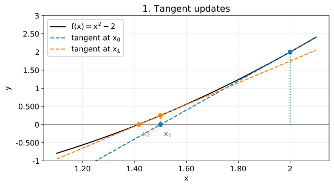
Figure 1 shows the first two updates for $f(x)=x^2-2$, starting from $x_0=2$.
def newton_history(f, df, x0, steps):
    """Run Newton iterations with an iteration limit, using either float or Decimal."""
    x = x0
    values = [x]
    for _ in range(steps):
        fx = f(x)
        if fx == 0:
            break
        slope = df(x)
        if slope == 0:
            raise ZeroDivisionError("Cannot update because the derivative is zero")
        x = x - fx / slope
        values.append(x)
    return values


def f(x):
    return x**2 - 2


def df(x):
    return 2 * x


xs_float = newton_history(f, df, 2.00, 7)
grid = np.linspace(1.10, 2.10, 400)
fig, ax = plt.subplots(figsize=(7, 4))
ax.plot(grid, f(grid), color="black", label=r"$f(x)=x^2-2$")
ax.axhline(0, color="gray", linewidth=1)
for n, color in enumerate(("tab:blue", "tab:orange")):
    xn, xn_next = xs_float[n:n + 2]
    ax.plot(grid, f(xn) + df(xn) * (grid - xn), "--",
            color=color, label=rf"tangent at $x_{n}$")
    ax.plot([xn, xn], [0, f(xn)], ":", color=color)
    ax.scatter([xn, xn_next], [f(xn), 0], color=color, zorder=3)
    ax.annotate(rf"$x_{n + 1}$", (xn_next, 0), xytext=(5, -18),
                textcoords="offset points", color=color)
ax.set(xlabel="$x$", ylabel="$y$", ylim=(-1, 3), title="1. Tangent updates")
ax.legend()
save_figure(fig, "01_tangents.svg")
2. The first-order error term cancels
A root $\alpha$ satisfying $f(\alpha)=0$ and $f^{\prime}(\alpha)\ne0$ is called a simple root. We also assume that $f$ is twice continuously differentiable in a neighborhood of $\alpha$.
Define the error as $e_n=x_n-\alpha$ and express $f(\alpha)$ using a Taylor expansion about $x_n$. The point $\xi_n$ in the remainder lies between $x_n$ and $\alpha$.
$$ \displaystyle \begin{aligned} 0&=f(\alpha)\\ &=f(x_n)+f^{\prime}(x_n)(\alpha-x_n)\\ &\quad+\frac{f^{\prime\prime}(\xi_n)}{2}(\alpha-x_n)^2\\ &=f(x_n)-f^{\prime}(x_n)e_n+\frac{f^{\prime\prime}(\xi_n)}{2}e_n^2. \end{aligned} $$
Rearranging and dividing by $f^{\prime}(x_n)$ gives
$$ \displaystyle \begin{aligned} f(x_n)&=f^{\prime}(x_n)e_n-\frac{f^{\prime\prime}(\xi_n)}{2}e_n^2,\\ \frac{f(x_n)}{f^{\prime}(x_n)}&=e_n-\frac{f^{\prime\prime}(\xi_n)}{2f^{\prime}(x_n)}e_n^2. \end{aligned} $$
Substituting this into the update formula gives
$$ \displaystyle \begin{aligned} e_{n+1}&=x_{n+1}-\alpha\\ &=x_n-\alpha-\frac{f(x_n)}{f^{\prime}(x_n)}\\ &=e_n-\left(e_n-\frac{f^{\prime\prime}(\xi_n)}{2f^{\prime}(x_n)}e_n^2\right)\\ &=\frac{f^{\prime\prime}(\xi_n)}{2f^{\prime}(x_n)}e_n^2. \end{aligned} $$
The $e_n$ in the update cancels the first-order term in $f(x_n)/f^{\prime}(x_n)$, leaving a term containing $e_n^2$. To establish quadratic convergence from this relation, we must also check that the iterates remain near the root and that the error tends to zero.
Starting points that guarantee convergence
Take a sufficiently small closed interval $I$ with $\alpha$ in its interior, such that $|f^{\prime}(x)|\ge m>0$ and $|f^{\prime\prime}(x)|\le M$ throughout the interval. Choose a positive constant $K\ge M/(2m)$ and then choose $\delta>0$ such that $[\alpha-\delta,\alpha+\delta]\subseteq I$ and $K\delta\le1/2$. If the initial error satisfies $|e_0|\le\delta$, the following holds:
$$ \displaystyle |e_{n+1}|\le K|e_n|^2\le\frac12|e_n|\le\delta $$
This follows by induction. The iterates remain in the interval and $e_n\to0$, so we do not need to assume convergence in advance.
Now suppose that $f^{\prime\prime}(\alpha)\ne0$ and that the iteration does not reach the root in finitely many steps. The following limit is then positive, and the convergence order is exactly two.
$$ \displaystyle \lim_{n\to\infty}\frac{|e_{n+1}|}{|e_n|^2} =\left|\frac{f^{\prime\prime}(\alpha)}{2f^{\prime}(\alpha)}\right|=C>0. $$
If $f^{\prime\prime}(\alpha)=0$, convergence can have an order higher than two, or the iteration can reach the root in finitely many steps. “At least quadratic” means that the next error is bounded by $K|e_n|^2$, while “exactly quadratic” means that the limit above is positive.
3. Checking the result with a square root
For $f(x)=x^2-2$ and $\alpha=\sqrt2$, we can simplify the error relation directly.
$$ \displaystyle \begin{aligned} x_{n+1}&=x_n-\frac{x_n^2-2}{2x_n} =\frac{x_n^2+2}{2x_n},\\ e_{n+1}&=\frac{x_n^2+2-2\alpha x_n}{2x_n}\\ &=\frac{x_n^2+\alpha^2-2\alpha x_n}{2x_n}\\ &=\frac{(x_n-\alpha)^2}{2x_n} =\frac{e_n^2}{2x_n},\\ C&=\frac{1}{2\sqrt2}\approx0.354. \end{aligned} $$
We also check this identity with SymPy. Use display() to show mathematical expressions.
x = sp.symbols("x", positive=True)
alpha_symbol = sp.sqrt(2)
next_error = x - (x**2 - 2) / (2 * x) - alpha_symbol
expected = (x - alpha_symbol)**2 / (2 * x)
assert sp.simplify(next_error - expected) == 0
display(Math(r"x-\frac{x^2-2}{2x}-\sqrt{2}=" + sp.latex(expected)))
display(Math(r"C=\frac{1}{2\sqrt{2}}\approx0.354"))
$$ \displaystyle x-\frac{x^2-2}{2x}-\sqrt{2}=\frac{\left(x - \sqrt{2}\right)^{2}}{2 x} $$
$$ \displaystyle C=\frac{1}{2\sqrt{2}}\approx0.354 $$
High-precision and ordinary floating-point calculations
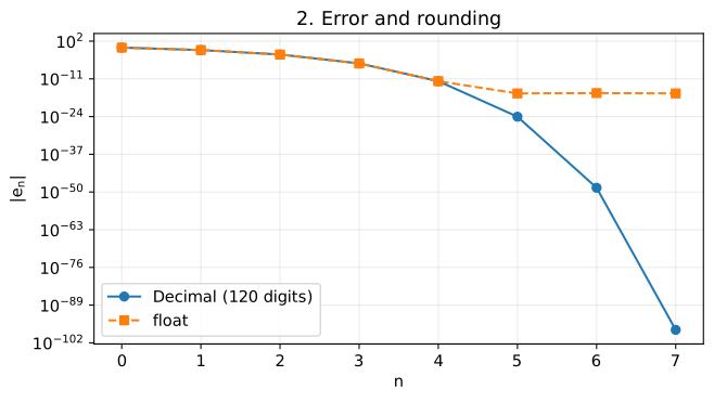
Compute $\sqrt2$ and the errors using Decimal with 120-digit precision. Evaluate the errors of the float approximations against the same reference value. Subtracting two float values can give zero even when an error remains, because the reference value is also rounded to float.
In Figure 2, the high-precision error decreases rapidly, while the float error levels off at about $10^{-16}$. The quadratic convergence derived here assumes arithmetic without rounding errors. With finite precision, rounding errors eventually prevent further error reduction.
alpha = Decimal(2).sqrt()
xs = newton_history(f, df, Decimal(2), 7)
errors = [abs(xn - alpha) for xn in xs]
float_errors = [abs(Decimal.from_float(xn) - alpha) for xn in xs_float]
ratios = [errors[n + 1] / errors[n]**2 for n in range(len(errors) - 1)]

# Format decimals in scientific notation with three significant digits, collect the results in a list, and display them with pprint.
rows = []
for n, (xn, error) in enumerate(zip(xs, errors)):
    rows.append({"n": n, "x_n": f"{xn:.2E}", "abs_error": f"{error:.2E}"})
pprint(rows, sort_dicts=False)

fig, ax = plt.subplots(figsize=(7, 4))
ax.semilogy(range(len(errors)), [float(e) for e in errors], "o-", label="Decimal (120 digits)")
ax.semilogy(range(len(float_errors)), [float(e) for e in float_errors], "s--", label="float")
ax.xaxis.set_major_locator(MaxNLocator(integer=True))
ax.set(xlabel="$n$", ylabel=r"$|e_n|$", title="2. Error and rounding")
ax.legend()
save_figure(fig, "02_errors.svg")
[{'n': 0, 'x_n': '2.00E+0', 'abs_error': '5.86E-1'},
 {'n': 1, 'x_n': '1.50E+0', 'abs_error': '8.58E-2'},
 {'n': 2, 'x_n': '1.42E+0', 'abs_error': '2.45E-3'},
 {'n': 3, 'x_n': '1.41E+0', 'abs_error': '2.12E-6'},
 {'n': 4, 'x_n': '1.41E+0', 'abs_error': '1.59E-12'},
 {'n': 5, 'x_n': '1.41E+0', 'abs_error': '8.99E-25'},
 {'n': 6, 'x_n': '1.41E+0', 'abs_error': '2.86E-49'},
 {'n': 7, 'x_n': '1.41E+0', 'abs_error': '2.89E-98'}]
Error ratios and convergence order
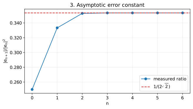
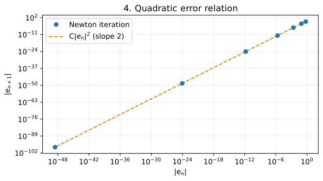
In Figure 3, the error ratio $|e_{n+1}|/|e_n|^2$ approaches the theoretical value $C=1/(2\sqrt2)$, about $0.354$. Figure 4 is a log-log plot with $|e_n|$ on the horizontal axis and $|e_{n+1}|$ on the vertical axis.
$$ \displaystyle \log|e_{n+1}|\approx\log C+2\log|e_n| $$
This relation explains why the points approach a straight line with slope two. We can also estimate the convergence order from three successive errors:
$$ \displaystyle p_n=\frac{\log(|e_{n+1}|/|e_n|)}{\log(|e_n|/|e_{n-1}|)} $$
This estimate also approaches two. In this example, the approximations look identical when displayed with three significant digits, but the error continues to decrease with each iteration.
constant = 1 / (2 * alpha)
orders = [
    (errors[n + 1] / errors[n]).ln() / (errors[n] / errors[n - 1]).ln()
    for n in range(1, len(errors) - 1)
]
pprint({"error_ratios": [f"{r:.2E}" for r in ratios],
        "estimated_orders": [f"{p:.2E}" for p in orders]}, sort_dicts=False)

fig, ax = plt.subplots(figsize=(7, 4))
ax.plot(range(len(ratios)), [float(r) for r in ratios], "o-", label="measured ratio")
ax.axhline(float(constant), color="tab:red", linestyle="--", label=r"$1/(2\sqrt{2})$")
ax.xaxis.set_major_locator(MaxNLocator(integer=True))
ax.set(xlabel="$n$", ylabel=r"$|e_{n+1}|/|e_n|^2$", title="3. Asymptotic error constant")
ax.legend()
save_figure(fig, "03_error_ratios.svg")

previous_errors = np.array([float(e) for e in errors[:-1]])
next_errors = np.array([float(e) for e in errors[1:]])
fig, ax = plt.subplots(figsize=(7, 4))
ax.loglog(previous_errors, next_errors, "o", label="Newton iteration", zorder=3)
ax.loglog(previous_errors, float(constant) * previous_errors**2, "--", label=r"$C|e_n|^2$ (slope 2)")
ax.set(xlabel=r"$|e_n|$", ylabel=r"$|e_{n+1}|$", title="4. Quadratic error relation")
ax.legend()
save_figure(fig, "04_error_relation.svg")
{'error_ratios': ['2.50E-1',
                  '3.33E-1',
                  '3.53E-1',
                  '3.54E-1',
                  '3.54E-1',
                  '3.54E-1',
                  '3.54E-1'],
 'estimated_orders': ['1.85E+0',
                      '1.98E+0',
                      '2.00E+0',
                      '2.00E+0',
                      '2.00E+0',
                      '2.00E+0']}
4. When convergence is not quadratic
Multiple roots give linear convergence
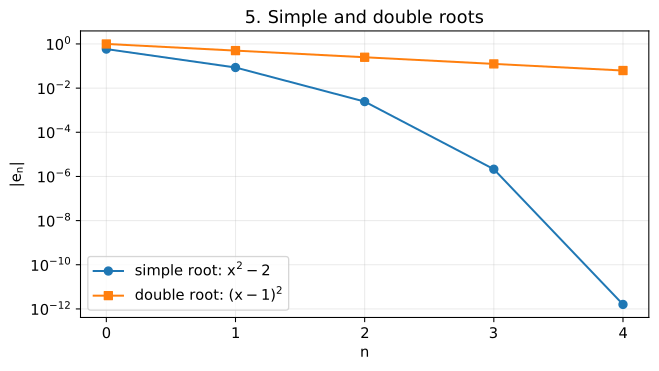
For $f(x)=(x-1)^2$, we have $f^{\prime}(1)=0$, so the simple-root condition does not hold. If $x_n\ne1$, the following relation holds.
$$ \displaystyle \begin{aligned} x_{n+1}&=x_n-\frac{(x_n-1)^2}{2(x_n-1)} =x_n-\frac{x_n-1}{2},\\ e_{n+1}&=x_n-1-\frac{x_n-1}{2}=\frac12e_n. \end{aligned} $$
The error halves at every iteration. More generally, for an integer $m\ge2$, the function $f(x)=(x-\alpha)^m$ gives $e_{n+1}=(1-1/m)e_n$. In Figure 5, the errors for the multiple root lie on a straight line when the vertical axis is logarithmic, because the error decreases by a fixed factor at every iteration.
multiple_xs = newton_history(lambda x: (x - 1)**2, lambda x: 2 * (x - 1), Decimal(2), 7)
multiple_errors = [abs(xn - 1) for xn in multiple_xs]
pprint({"multiple_root_ratios": [
    f"{multiple_errors[n + 1] / multiple_errors[n]:.2E}"
    for n in range(len(multiple_errors) - 1)
]})

# Compare the first five points to make the linear decrease at the multiple root easier to see.
fig, ax = plt.subplots(figsize=(7, 4))
ax.semilogy(range(5), [float(e) for e in errors[:5]], "o-", label=r"simple root: $x^2-2$")
ax.semilogy(range(5), [float(e) for e in multiple_errors[:5]], "s-", label=r"double root: $(x-1)^2$")
ax.xaxis.set_major_locator(MaxNLocator(integer=True))
ax.set(xlabel="$n$", ylabel=r"$|e_n|$", title="5. Simple and double roots")
ax.legend()
save_figure(fig, "05_multiple_root.svg")
{'multiple_root_ratios': ['5.00E-1',
                          '5.00E-1',
                          '5.00E-1',
                          '5.00E-1',
                          '5.00E-1',
                          '5.00E-1',
                          '5.00E-1']}
Some starting points do not lead to convergence
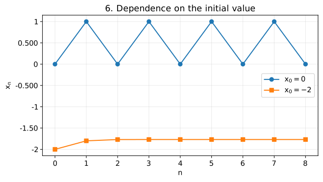
For $f(x)=x^3-2x+2$, starting from $x_0=0$ gives
$$ \displaystyle x_1=0-\frac{2}{-2}=1,\qquad x_2=1-\frac{1}{1}=0 $$
The iterates alternate between zero and one. Figure 6 compares this sequence with one starting from $x_0=-2$, which converges to the root. Even if the derivative is nonzero, convergence is not guaranteed when the starting point is far from the root.
def cubic(x):
    return x**3 - 2 * x + 2


def cubic_derivative(x):
    return 3 * x**2 - 2


cycle = newton_history(cubic, cubic_derivative, Decimal(0), 8)
convergent = newton_history(cubic, cubic_derivative, Decimal(-2), 8)
pprint({"x0=0": [f"{xn:.2E}" if xn != 0 else "0" for xn in cycle],
        "x0=-2, final": f"{convergent[-1]:.2E}"}, sort_dicts=False)

fig, ax = plt.subplots(figsize=(7, 4))
ax.plot(range(len(cycle)), [float(xn) for xn in cycle], "o-", label=r"$x_0=0$")
ax.plot(range(len(convergent)), [float(xn) for xn in convergent], "s-", label=r"$x_0=-2$")
ax.xaxis.set_major_locator(MaxNLocator(integer=True))
ax.set(xlabel="$n$", ylabel="$x_n$", title="6. Dependence on the initial value")
ax.legend()
save_figure(fig, "06_initial_values.svg")
{'x0=0': ['0', '1.00E+0', '0', '1.00E+0', '0', '1.00E+0', '0', '1.00E+0', '0'],
 'x0=-2, final': '-1.77E+0'}
Conclusion
In Newton’s method, the first-order error term cancels in the update formula. If the function is twice continuously differentiable and the iteration starts close enough to a simple root, convergence is at least quadratic. If the root is not reached in finitely many steps and $f^{\prime\prime}(\alpha)\ne0$, the convergence order is exactly two, with asymptotic error constant $|f^{\prime\prime}(\alpha)/(2f^{\prime}(\alpha))|$.
The square-root calculation confirmed this error constant and convergence order numerically. Multiple roots give slower convergence, and some starting points do not lead to convergence at all. With finite precision, rounding errors can also stop the error from decreasing.