Examples of Newton’s method failing to converge in Python (Rewritten from an earlier blog post)
Environment
Python 3.14.6, NumPy 2.5.4, SciPy 1.18.1, Matplotlib 3.11.2 (Jupyter Notebook).
This article is a rewrite of a post from around 2013–2016, with calculations performed in the environment described above.
Overview
Newton’s method solves $f(x)=0$ iteratively, using the $x$ coordinate where a tangent line meets the horizontal axis as the next approximation.
We reproduce three cases in Python: iterates that alternate between two points, iterates that keep moving away from the root, and an update that cannot proceed because the derivative is zero. We explain each failure from the update formula and plot the functions, tangent lines, iterates, and residuals. Finally, we compare changing the starting point with using Brent’s method.
Setup
Run the code in Jupyter Notebook from top to bottom. Round numbers to three significant digits only when displaying them.
import platform
from pathlib import Path
from pprint import pprint

import matplotlib
import matplotlib.pyplot as plt
import numpy as np
import scipy
from IPython.display import Math, display
from matplotlib.ticker import FuncFormatter, MaxNLocator
from matplotlib_inline.backend_inline import set_matplotlib_formats
from scipy.optimize import brentq, newton

%matplotlib inline
set_matplotlib_formats("svg")

print("Python:", platform.python_version())
print("NumPy:", np.__version__)
print("SciPy:", scipy.__version__)
print("Matplotlib:", matplotlib.__version__)

# Display decimals in arrays and axis ticks with three significant digits.
np.set_printoptions(formatter={"float_kind": lambda x: f"{x:#.3g}"})
plt.rcParams.update({"font.size": 11, "axes.grid": True, "grid.alpha": 0.250})
output_dir = Path("102_nb_files")
output_dir.mkdir(exist_ok=True)


def save_figure(fig, filename, iteration=False):
    for ax in fig.axes:
        ax.xaxis.set_major_formatter(FuncFormatter(lambda x, pos: f"{x:#.3g}"))
        ax.yaxis.set_major_formatter(FuncFormatter(lambda y, pos: f"{y:#.3g}"))
        if iteration:
            ax.xaxis.set_major_locator(MaxNLocator(integer=True))
            ax.xaxis.set_major_formatter(FuncFormatter(lambda x, pos: f"{x:.0f}"))
    fig.savefig(output_dir / filename, format="svg", bbox_inches="tight")
    plt.show()
    plt.close(fig)
Python: 3.14.6
NumPy: 2.5.4
SciPy: 1.18.1
Matplotlib: 3.11.2
1. The update formula and stopping conditions
Let $t_n(x)$ be the tangent line at $(x_n,f(x_n))$. Near $x_n$, we can approximate $f(x)$ as follows.
$$ \displaystyle t_n(x)=f(x_n)+f^{\prime}(x_n)(x-x_n)\approx f(x) $$
Take the $x$ coordinate where the tangent meets the horizontal axis as the next approximation, $x_{n+1}$. If $f^{\prime}(x_n)\ne0$, rearranging gives
$$ \displaystyle \begin{gathered} 0=f(x_n)+f^{\prime}(x_n)(x_{n+1}-x_n),\\ x_{n+1}-x_n=-\frac{f(x_n)}{f^{\prime}(x_n)},\\ x_{n+1}=x_n-\frac{f(x_n)}{f^{\prime}(x_n)}. \end{gathered} $$
If $f$ is twice continuously differentiable near a root $r$ and $f^{\prime}(r)\ne0$, the method converges at least quadratically from a starting point sufficiently close to $r$. However, it does not converge from every starting point.
The function newton_trace below stores the initial value and every iterate, stopping when the residual $|f(x_n)|$ is at most $1.00\times10^{-10}$. It also returns a stopping reason if the derivative becomes zero or the iteration limit is reached. The residual tolerance is chosen for these examples. For other problems, adjust it to the scale of the function values and the required accuracy.
def newton_trace(f, df, x0, maxiter=12, ftol=1.00e-10):
    """Return the iteration history, including the initial value, and the stopping reason."""
    x = float(x0)
    history = [x]
    for n in range(maxiter + 1):
        fx = float(f(x))
        if not np.isfinite(fx):
            reason = "Function value is not finite"
            break
        if abs(fx) <= ftol:
            reason = "Residual is within tolerance"
            break
        if n == maxiter:
            reason = "Iteration limit reached"
            break
        dfx = float(df(x))
        if not np.isfinite(dfx) or dfx == 0:
            reason = "Derivative is zero or not finite"
            break
        # Check the residual before dividing to avoid unnecessary division at a root.
        x_next = x - fx / dfx
        if not np.isfinite(x_next):
            reason = "Updated value is not finite"
            break
        history.append(x_next)
        x = x_next
    return np.array(history), reason


display(Math(r"x_{n+1}=x_n-\frac{f(x_n)}{f'(x_n)}"))
$$ \displaystyle x_{n+1}=x_n-\frac{f(x_n)}{f^{\prime}(x_n)} $$
2. Alternating between zero and one
Set $f(x)=x^3-2x+2$ and $f^{\prime}(x)=3x^2-2$, and start from $x_0=0$.
$$ \displaystyle \begin{aligned} f(0)&=2,\qquad f^{\prime}(0)=-2,\\ x_1&=0-\frac{2}{-2}=1,\\ f(1)&=1-2+2=1,\\ f^{\prime}(1)&=3-2=1,\\ x_2&=1-\frac{1}{1}=0. \end{aligned} $$
Two updates return to the starting point, so $x_{2k}=0$ and $x_{2k+1}=1$ for $k=0,1,2,\ldots$. Neither point is a root, and the residual alternates between two and one. This is a cycle of period two that occurs even in exact arithmetic; it is not caused by rounding errors.
def f_cycle(x):
    return x**3 - 2 * x + 2


def df_cycle(x):
    return 3 * x**2 - 2


cycle, cycle_reason = newton_trace(f_cycle, df_cycle, 0)
print(cycle_reason)
pprint(cycle)
pprint(np.abs(f_cycle(cycle)))

# Each tangent's intersection with the horizontal axis gives the next iterate.
grid = np.linspace(-2, 2, 401)
fig, ax = plt.subplots(figsize=(8, 5), layout="constrained")
ax.plot(grid, f_cycle(grid), label=r"$f(x)=x^3-2x+2$")
ax.plot(grid, 2 - 2 * grid, "--", label=r"$t_0(x)=2-2x$")
ax.plot(grid, grid, "--", label=r"$t_1(x)=x$")
ax.axhline(0, color="black", linewidth=1)
ax.scatter([0, 1], [2, 1], color="black", zorder=5)
ax.scatter([1, 0], [0, 0], color="tab:red", zorder=5)
ax.set(xlabel="$x$", ylabel="$y$", title="Two-cycle: tangent intersections")
ax.legend()
save_figure(fig, "01_cycle_tangents.svg")

fig, axes = plt.subplots(1, 2, figsize=(10, 4), layout="constrained")
steps = np.arange(cycle.size)
axes[0].plot(steps, cycle, "o-")
axes[0].set(xlabel="$n$", ylabel="$x_n$", title="Iterates: 0, 1, 0, 1, ...")
axes[1].plot(steps, np.abs(f_cycle(cycle)), "o-", color="tab:orange")
axes[1].set(xlabel="$n$", ylabel=r"$|f(x_n)|$", title="Residual: 2, 1, 2, 1, ...")
save_figure(fig, "02_cycle_history.svg", iteration=True)
Iteration limit reached
array([0.00, 1.00, 0.00, 1.00, 0.00, 1.00, 0.00, 1.00, 0.00, 1.00, 0.00,
       1.00, 0.00])
array([2.00, 1.00, 2.00, 1.00, 2.00, 1.00, 2.00, 1.00, 2.00, 1.00, 2.00,
       1.00, 2.00])
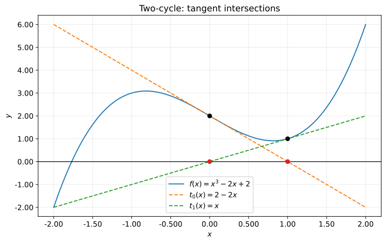
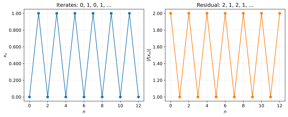
A tangent can be drawn at every step, but the iterates alternate between zero and one and the residual does not approach zero. Looking at several iterates, instead of only the final value, reveals this cycle.
3. Absolute values that double at every step
Next, consider $f(x)=\sqrt[3]{x}$, the real cube-root function. Its root is $r=0$. Setting $y=\sqrt[3]{x}$ gives $x=y^3$, so for $x\ne0$ we obtain
$$ \displaystyle \begin{aligned} \frac{dx}{dy}&=3y^2,\\ f^{\prime}(x)&=\frac{dy}{dx}=\frac{1}{3y^2} =\frac{1}{3(\sqrt[3]{x})^2}. \end{aligned} $$
Assuming $x_n\ne0$, substitute this into the update formula.
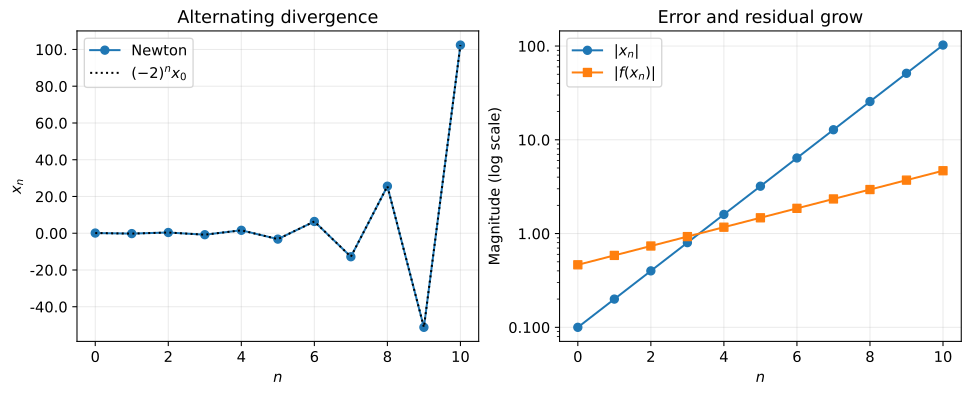
$$ \displaystyle \begin{aligned} x_{n+1} &=x_n-\frac{\sqrt[3]{x_n}}{\frac{1}{3(\sqrt[3]{x_n})^2}}\\ &=x_n-3(\sqrt[3]{x_n})^3\\ &=x_n-3x_n=-2x_n,\\ x_n&=(-2)^n x_0,\qquad |x_n|=2^n|x_0|. \end{aligned} $$
If $x_0\ne0$, the iterates alternate in sign while moving away from the root. The residual $|f(x_n)|=2^{n/3}|x_0|^{1/3}$ also keeps growing. At the root $r=0$, $f$ is not differentiable, so the local convergence conditions in Section 1 do not hold. The implementation uses np.cbrt to compute real cube roots for negative inputs as well.
def f_diverge(x):
    return np.cbrt(x)


def df_diverge(x):
    return 1 / (3 * np.cbrt(x)**2)


diverging, diverging_reason = newton_trace(f_diverge, df_diverge, 0.100, maxiter=10)
print(diverging_reason)
pprint(diverging)

steps = np.arange(diverging.size)
theory = 0.100 * (-2)**steps
fig, axes = plt.subplots(1, 2, figsize=(10, 4), layout="constrained")
axes[0].plot(steps, diverging, "o-", label="Newton")
axes[0].plot(steps, theory, ":", color="black", label=r"$(-2)^n x_0$")
axes[0].set(xlabel="$n$", ylabel="$x_n$", title="Alternating divergence")
axes[0].legend()
axes[1].semilogy(steps, np.abs(diverging), "o-", label=r"$|x_n|$")
axes[1].semilogy(steps, np.abs(f_diverge(diverging)), "s-", label=r"$|f(x_n)|$")
axes[1].set(xlabel="$n$", ylabel="Magnitude (log scale)", title="Error and residual grow")
axes[1].legend()
save_figure(fig, "03_divergence.svg", iteration=True)
Iteration limit reached
array([0.100, -0.200, 0.400, -0.800, 1.60, -3.20, 6.40, -12.8, 25.6,
       -51.2, 102.])
4. A zero derivative prevents an update
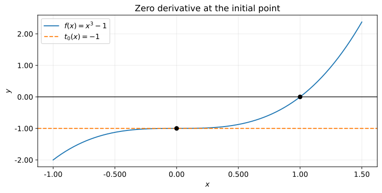
The function $f(x)=x^3-1$ has a root at $r=1$, but starting from $x_0=0$ gives
$$ \displaystyle f(0)=-1,\qquad f^{\prime}(0)=3\cdot0^2=0 $$
The denominator in the update formula is zero, so the next approximation $x_1$ cannot be computed. The tangent is $y=-1$ and does not meet the horizontal axis.
Our newton_trace function stops before dividing by zero and returns the reason. A zero derivative is not a problem if $f(x_n)=0$, because the root has already been reached. To avoid unnecessary division in that case, the code checks the residual before the derivative.
def f_flat(x):
    return x**3 - 1


def df_flat(x):
    return 3 * x**2


stopped, stopped_reason = newton_trace(f_flat, df_flat, 0)
print(stopped_reason)
pprint(stopped)

grid = np.linspace(-1, 1.50, 301)
fig, ax = plt.subplots(figsize=(8, 4), layout="constrained")
ax.plot(grid, f_flat(grid), label=r"$f(x)=x^3-1$")
ax.axhline(-1, linestyle="--", color="tab:orange", label=r"$t_0(x)=-1$")
ax.axhline(0, color="black", linewidth=1)
ax.scatter([0, 1], [-1, 0], color="black", zorder=5)
ax.set(xlabel="$x$", ylabel="$y$", title="Zero derivative at the initial point")
ax.legend()
save_figure(fig, "04_zero_derivative.svg")
Derivative is zero or not finite
array([0.00])
5. Comparing starting points and methods
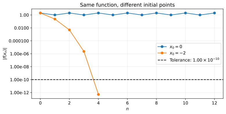
For the function $f(x)=x^3-2x+2$ from Section 2, changing the starting point to $x_0=-2$ gives convergence. Keeping $x_0=0$ and increasing the iteration limit does not remove the cycle between zero and one.
To use Newton’s method with SciPy’s newton, pass the derivative through the fprime argument. Omitting fprime selects the secant method. Here we set disp=False and full_output=True to receive the final value and convergence status even if the method fails to converge.
Our newton_trace uses the residual as its stopping criterion, while SciPy’s newton uses the step size $|x_{n+1}-x_n|$. The official SciPy documentation also calls for checking the result, so we inspect the residual as well as the convergence status.
This polynomial is continuous, and its values at the interval endpoints are
$$ \displaystyle \begin{aligned} f(-2)&=-8+4+2=-2<0,\\ f(-1)&=-1+2+2=3>0. \end{aligned} $$
The opposite signs imply that the interval $[-2,-1]$ contains at least one root. Brent’s method can also be used when a function is continuous on an interval and has opposite signs at its endpoints. We display the root with three significant digits but compute the residual before rounding.
converging, converging_reason = newton_trace(f_cycle, df_cycle, -2)
print(converging_reason)

# Show the convergence flag and residual instead of treating an unconverged result as a root.
failed_x, failed_info = newton(
    f_cycle, 0, fprime=df_cycle, maxiter=12, full_output=True, disp=False
)
brent_x, brent_info = brentq(f_cycle, -2, -1, full_output=True)
pprint({
    "Newton x0=0": {
        "converged": failed_info.converged,
        "last_x": f"{failed_x:#.3g}",
        "residual": f"{abs(f_cycle(failed_x)):#.3g}",
    },
    "Newton x0=-2": {
        "last_x": f"{converging[-1]:#.3g}",
        "residual": f"{abs(f_cycle(converging[-1])):#.3g}",
    },
    "Brent [-2, -1]": {
        "converged": brent_info.converged,
        "root": f"{brent_x:#.3g}",
        "residual": f"{abs(f_cycle(brent_x)):#.3g}",
    },
}, sort_dicts=False)
display(Math(r"\hat{x}_{\mathrm{Brent}}\approx " + f"{brent_x:#.3g}"))

fig, ax = plt.subplots(figsize=(8, 4), layout="constrained")
for values, label in [(cycle, "$x_0=0$"), (converging, "$x_0=-2$")]:
    ax.semilogy(np.arange(values.size), np.abs(f_cycle(values)), "o-", label=label)
ax.axhline(1.00e-10, linestyle="--", color="black", label=r"Tolerance: $1.00\times10^{-10}$")
ax.set(xlabel="$n$", ylabel=r"$|f(x_n)|$", title="Same function, different initial points")
ax.legend()
save_figure(fig, "05_initial_values.svg", iteration=True)
Residual is within tolerance
{'Newton x0=0': {'converged': False, 'last_x': '0.00', 'residual': '2.00'},
 'Newton x0=-2': {'last_x': '-1.77', 'residual': '5.05e-13'},
 'Brent [-2, -1]': {'converged': True, 'root': '-1.77', 'residual': '1.33e-15'}}
$$ \displaystyle \hat{x}_{\mathrm{Brent}}\approx -1.77 $$
Conclusion
We examined three failures of Newton’s method using the update formulas and iteration histories computed in Python.
In the cycle between zero and one, the residual did not approach zero. In the cube-root example, the iterates kept moving away from the root. With a zero derivative, the update denominator was zero, preventing the next approximation from being computed.
Before using a computed value as a root, check the residual, derivative, and stopping reason as well as the final value. A different starting point may lead to convergence. Brent’s method is another option when the function is continuous on an interval and its endpoint values have opposite signs.