What does BFGS approximate without computing the Hessian? (Rewritten from an earlier blog post)
Environment
Python 3.14.6, NumPy 2.5.4, SciPy 1.18.1, Matplotlib 3.11.2.
This article is a rewrite of a post from around 2013–2016, with calculations performed in the environment described above.
Overview
BFGS is a quasi-Newton method that approximates the Hessian or its inverse using changes in position and gradient. It does not compute each second derivative directly. Instead, it updates a matrix with the curvature observed along the step direction.
We derive the secant condition and BFGS updates, then implement them in Python. Quadratic and Rosenbrock examples let us examine solution convergence, matrix approximation error, and the secant residual separately.
Setup
Run the code in Jupyter Notebook from top to bottom.
Imports and plotting setup
import platform
import sys
from importlib.metadata import version
from pathlib import Path
from pprint import pprint

import matplotlib.pyplot as plt
import numpy as np
from IPython.display import Latex, Math, SVG, display
from matplotlib.ticker import FuncFormatter, MaxNLocator, NullFormatter
from matplotlib_inline.backend_inline import set_matplotlib_formats
from scipy.optimize import line_search, minimize

%matplotlib inline
set_matplotlib_formats("svg")

assert platform.python_version() == "3.14.6"
assert sys.prefix != sys.base_prefix
print("Environment: wa-src(3.14.6)")
print("Python:", platform.python_version())
print("OS:", platform.platform())
print("Executable:", sys.executable)
pprint({name: version(name) for name in ("numpy", "scipy", "matplotlib")})

np.set_printoptions(formatter={"float_kind": lambda v: f"{v:#.3g}"})
plt.rcParams.update({"font.size": 11, "svg.fonttype": "none"})
figure_dir = Path("103_nb_files")
figure_dir.mkdir(exist_ok=True)


def save_figure(fig, name):
    """Format decimal ticks to three digits, save the SVG, and display it."""
    for ax in fig.axes:
        for axis in (ax.xaxis, ax.yaxis):
            axis.set_major_formatter(FuncFormatter(lambda v, _: f"{v:#.3g}"))
            axis.set_minor_formatter(NullFormatter())
        if ax.get_xlabel() == "Iteration":
            ax.xaxis.set_major_locator(MaxNLocator(integer=True))
            ax.xaxis.set_major_formatter(FuncFormatter(lambda v, _: f"{v:.0f}"))
        ax.grid(alpha=0.250)
        if ax.get_legend_handles_labels()[0]:
            ax.legend()
    path = figure_dir / name
    fig.savefig(path, format="svg", bbox_inches="tight")
    plt.close(fig)
    display(SVG(filename=str(path)))
Environment: wa-src(3.14.6)
Python: 3.14.6
OS: macOS-26.5.2-arm64-arm-64bit-Mach-O
Executable: /Users/hiroshi/private/wa_src/.venv/bin/python
{'matplotlib': '3.11.2', 'numpy': '2.5.4', 'scipy': '1.18.1'}
1. Approximating the curvature of a quadratic model
We minimize $f:\mathbb{R}^n\to\mathbb{R}$. Assume $f$ is twice continuously differentiable, and write its gradient as $\mathbf{g}_k=\nabla f(\mathbf{x}_k)$ and its true Hessian as $\mathbf{G}_k=\nabla^2f(\mathbf{x}_k)$. The Taylor expansion is
$$ f(\mathbf{x}_k+\mathbf{p}) =f(\mathbf{x}_k)+\mathbf{g}_k^\top\mathbf{p} +\frac12\mathbf{p}^\top\mathbf{G}_k\mathbf{p} +o(\|\mathbf{p}\|^2) $$
Replace $\mathbf{G}_k$ with a symmetric positive definite matrix $\mathbf{B}_k$ to form the quadratic model $q_k$.
$$ \begin{aligned} q_k(\mathbf{p})&=f(\mathbf{x}_k)+\mathbf{g}_k^\top\mathbf{p} +\frac12\mathbf{p}^\top\mathbf{B}_k\mathbf{p},\\ \nabla_{\mathbf{p}}q_k(\mathbf{p})&=\mathbf{g}_k+\mathbf{B}_k\mathbf{p},\\ \nabla_{\mathbf{p}}q_k(\mathbf{p}_k)=\mathbf{0} &\Longrightarrow \mathbf{B}_k\mathbf{p}_k=-\mathbf{g}_k,\\ \mathbf{p}_k&=-\mathbf{H}_k\mathbf{g}_k, \qquad \mathbf{H}_k=\mathbf{B}_k^{-1},\\ \mathbf{x}_{k+1}&=\mathbf{x}_k+\alpha_k\mathbf{p}_k. \end{aligned} $$
$\mathbf{B}_k$ approximates the Hessian, and $\mathbf{H}_k$ approximates its inverse. Here, $\mathbf{H}$ is not the Hessian itself. Where $\mathbf{G}_k$ is indefinite, a positive definite $\mathbf{B}_k$ cannot reproduce the negative curvature.
2. What gradient differences tell us
Define the step and gradient difference by
$$ \mathbf{s}_k=\mathbf{x}_{k+1}-\mathbf{x}_k, \qquad \mathbf{y}_k=\mathbf{g}_{k+1}-\mathbf{g}_k $$
Differentiate the gradient along the line segment with respect to $t$, then integrate to obtain the following relation.
$$ \begin{aligned} \frac{d}{dt}\nabla f(\mathbf{x}_k+t\mathbf{s}_k) &=\nabla^2f(\mathbf{x}_k+t\mathbf{s}_k)\mathbf{s}_k,\\ \mathbf{y}_k &=\int_0^1\nabla^2f(\mathbf{x}_k+t\mathbf{s}_k)\mathbf{s}_k\,dt,\\ \overline{\mathbf{G}}_k &=\int_0^1\nabla^2f(\mathbf{x}_k+t\mathbf{s}_k)\,dt,\\ \mathbf{y}_k&=\overline{\mathbf{G}}_k\mathbf{s}_k. \end{aligned} $$
The observation is the action of the average Hessian along the segment on $\mathbf{s}_k$. In general, $\mathbf{y}_k=\mathbf{G}_k\mathbf{s}_k$ does not hold. Requiring the approximate matrix to satisfy this observed relation gives the secant condition.
$$ \boxed{\mathbf{B}_{k+1}\mathbf{s}_k=\mathbf{y}_k} \qquad\Longleftrightarrow\qquad \boxed{\mathbf{H}_{k+1}\mathbf{y}_k=\mathbf{s}_k} $$
This condition gives $n$ equations. A symmetric matrix has $n(n+1)/2$ unknown entries, so for $n\gt 1$ it does not determine the whole matrix. One step provides curvature information along that direction, not full matrix information.
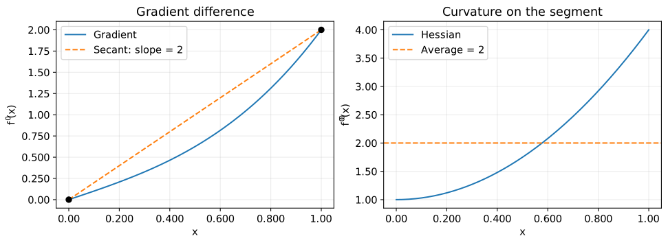
Consider the scalar function $f(x)=x^4/4+x^2/2$, with a move from $x_0=0$ to $x_1=1$.
$$ \begin{aligned} f^{\prime}(x)&=x^3+x,\qquad f^{\prime\prime}(x)=3x^2+1,\\ \frac{y}{s}&=\frac{f^{\prime}(1)-f^{\prime}(0)}{1-0}=2,\\ \int_0^1f^{\prime\prime}(t)\,dt&=[t^3+t]_0^1=2,\\ f^{\prime\prime}(0)&=1,\qquad f^{\prime\prime}(1)=4. \end{aligned} $$
The secant slope in Figure 1 is 2, different from the second derivatives at either endpoint.
x = np.linspace(0, 1, 200)
fig, axes = plt.subplots(1, 2, figsize=(10, 3.60), layout="constrained")
axes[0].plot(x, x**3 + x, label="Gradient")
axes[0].plot(x, 2*x, "--", label="Secant: slope = 2")
axes[0].scatter([0, 1], [0, 2], color="black", zorder=3)
axes[0].set(xlabel="$x$", ylabel="$f'(x)$", title="Gradient difference")
axes[1].plot(x, 3*x**2 + 1, label="Hessian")
axes[1].axhline(2, color="tab:orange", linestyle="--", label="Average = 2")
axes[1].set(xlabel="$x$", ylabel="$f''(x)$", title="Curvature on the segment")
save_figure(fig, "01_secant.svg")
3. Constructing the BFGS update
Drop the subscript $k$ and use $+$ for the updated matrix. Choose the following two outer products as a correction that preserves symmetry.
$$ \mathbf{B}_{+}=\mathbf{B} +a\mathbf{y}\mathbf{y}^\top +b(\mathbf{B}\mathbf{s})(\mathbf{B}\mathbf{s})^\top. $$
Multiply on the right by $\mathbf{s}$ and collect the coefficients.
$$ \begin{aligned} \mathbf{B}_{+}\mathbf{s} &=\mathbf{B}\mathbf{s} +a\mathbf{y}(\mathbf{y}^\top\mathbf{s}) +b\mathbf{B}\mathbf{s}(\mathbf{s}^\top\mathbf{B}\mathbf{s})\\ &=(1+b\mathbf{s}^\top\mathbf{B}\mathbf{s})\mathbf{B}\mathbf{s} +a(\mathbf{s}^\top\mathbf{y})\mathbf{y}. \end{aligned} $$
Set the coefficient of $\mathbf{B}\mathbf{s}$ to zero and that of $\mathbf{y}$ to one.
$$ \begin{aligned} 1+b\mathbf{s}^\top\mathbf{B}\mathbf{s}=0 &\Longrightarrow b=-\frac{1}{\mathbf{s}^\top\mathbf{B}\mathbf{s}},\\ a\mathbf{s}^\top\mathbf{y}=1 &\Longrightarrow a=\frac{1}{\mathbf{s}^\top\mathbf{y}},\\ \mathbf{B}_{+} &=\mathbf{B} -\frac{\mathbf{B}\mathbf{s}\mathbf{s}^\top\mathbf{B}} {\mathbf{s}^\top\mathbf{B}\mathbf{s}} +\frac{\mathbf{y}\mathbf{y}^\top}{\mathbf{s}^\top\mathbf{y}},\\ \mathbf{B}_{+}\mathbf{s} &=\mathbf{B}\mathbf{s}-\mathbf{B}\mathbf{s}+\mathbf{y}=\mathbf{y}. \end{aligned} $$
This is the BFGS update for the Hessian approximation. It adds and subtracts two rank-one matrices, so the change has rank at most two. The secant condition alone does not uniquely determine this update; it follows from the chosen correction form.
Updating the inverse directly
With $\rho=1/(\mathbf{s}^\top\mathbf{y})$, the equivalent inverse update is
$$ \mathbf{H}_{+} =(\mathbf{I}-\rho\mathbf{s}\mathbf{y}^\top) \mathbf{H} (\mathbf{I}-\rho\mathbf{y}\mathbf{s}^\top) +\rho\mathbf{s}\mathbf{s}^\top $$
The inverse relation can be checked by verifying $\mathbf{B}_{+}\mathbf{H}_{+}=\mathbf{I}$. We can also check the secant condition directly.
$$ \begin{aligned} (\mathbf{I}-\rho\mathbf{y}\mathbf{s}^\top)\mathbf{y} &=\mathbf{y}-\rho\mathbf{y}(\mathbf{s}^\top\mathbf{y})=\mathbf{0},\\ \mathbf{H}_{+}\mathbf{y} &=\mathbf{0}+\rho\mathbf{s}(\mathbf{s}^\top\mathbf{y})=\mathbf{s}. \end{aligned} $$
In the implementation, expand the products to avoid matrix–matrix multiplication.
$$ \begin{aligned} \mathbf{v}&=\mathbf{H}\mathbf{y},\\ \mathbf{H}_{+} &=\mathbf{H}-\rho\mathbf{s}\mathbf{y}^\top\mathbf{H} -\rho\mathbf{H}\mathbf{y}\mathbf{s}^\top +\rho^2\mathbf{s}(\mathbf{y}^\top\mathbf{H}\mathbf{y})\mathbf{s}^\top +\rho\mathbf{s}\mathbf{s}^\top\\ &=\mathbf{H}-\rho(\mathbf{s}\mathbf{v}^\top+\mathbf{v}\mathbf{s}^\top) +\rho(1+\rho\mathbf{y}^\top\mathbf{v})\mathbf{s}\mathbf{s}^\top. \end{aligned} $$
Matrix storage and each update cost $O(n^2)$. There is no need to compute an inverse at every step. To guard against rounding effects, we skip an update when $\mathbf{s}^\top\mathbf{y}$ is at most $1.00\times10^{-12}\|\mathbf{s}\|\|\mathbf{y}\|$. This threshold is an implementation choice.
def inverse_bfgs(H, s, y):
    """Update the inverse Hessian approximation; keep the previous matrix for small curvature."""
    sy = s @ y
    if sy <= 1.00e-12 * np.linalg.norm(s) * np.linalg.norm(y):
        return H.copy(), False
    rho = 1 / sy
    v = H @ y
    updated = H + rho * (1 + rho * (y @ v)) * np.outer(s, s)
    updated -= rho * (np.outer(s, v) + np.outer(v, s))
    # Remove asymmetry introduced by floating-point arithmetic.
    return (updated + updated.T) / 2, True


display(Latex(r"\(\displaystyle\boxed{\mathbf{p}_k=-\mathbf{H}_k\mathbf{g}_k,"
              r"\quad \mathbf{H}_{k+1}\mathbf{y}_k=\mathbf{s}_k}\)"))
$$ \displaystyle\boxed{\mathbf{p}_k=-\mathbf{H}_k\mathbf{g}_k,\quad \mathbf{H}_{k+1}\mathbf{y}_k=\mathbf{s}_k} $$
4. Positive definiteness and line search
If $\mathbf{H}\succ0$ and $\mathbf{s}^\top\mathbf{y}\gt 0$, the updated matrix remains positive definite. Let $\mathbf{V}=\mathbf{I}-\rho\mathbf{s}\mathbf{y}^\top$. For any $\mathbf{z}\ne\mathbf{0}$,
$$ \mathbf{z}^\top\mathbf{H}_{+}\mathbf{z} =(\mathbf{V}^\top\mathbf{z})^\top\mathbf{H}(\mathbf{V}^\top\mathbf{z}) +\rho(\mathbf{s}^\top\mathbf{z})^2. $$
If $\mathbf{s}^\top\mathbf{z}\ne0$, the second term is positive. If $\mathbf{s}^\top\mathbf{z}=0$, then $\mathbf{V}^\top\mathbf{z}=\mathbf{z}$ and the first term is positive. Thus the search direction is a descent direction whenever the gradient is nonzero.
$$ \mathbf{g}_k^\top\mathbf{p}_k =-\mathbf{g}_k^\top\mathbf{H}_k\mathbf{g}_k\lt 0. $$
Even along a descent direction, an overly large step length $\alpha_k$ can increase the function value. The Wolfe conditions used in line search are, for $0\lt c_1\lt c_2\lt 1$,
$$ \begin{aligned} f(\mathbf{x}_k+\alpha_k\mathbf{p}_k) &\le f(\mathbf{x}_k)+c_1\alpha_k\mathbf{g}_k^\top\mathbf{p}_k,\\ \mathbf{g}_{k+1}^\top\mathbf{p}_k &\ge c_2\mathbf{g}_k^\top\mathbf{p}_k \end{aligned} $$
The second condition gives the positive curvature condition below.
$$ \begin{aligned} \mathbf{s}_k^\top\mathbf{y}_k &=\alpha_k\mathbf{p}_k^\top(\mathbf{g}_{k+1}-\mathbf{g}_k)\\ &\ge\alpha_k(c_2-1)\mathbf{g}_k^\top\mathbf{p}_k\gt 0. \end{aligned} $$
SciPy’s line_search uses the strong Wolfe conditions, replacing the second inequality with $|\mathbf{g}_{k+1}^\top\mathbf{p}_k|\le c_2|\mathbf{g}_k^\top\mathbf{p}_k|$. This also implies the curvature condition above. See the SciPy documentation.
The following implementation records the iteration history. It stops when $\|\mathbf{g}_k\|_2\le1.00\times10^{-8}$. A failed line search raises an exception; reaching the iteration limit returns success=False. The step argument supplies an exact step length only for the quadratic experiment.
def bfgs_trace(f, grad, x0, step=None, tol=1.00e-8, maxiter=200):
    x = np.array(x0, dtype=float)
    H = np.eye(x.size)
    xs, matrices, residuals, accepted = [x.copy()], [H.copy()], [], []
    for _ in range(maxiter):
        g = grad(x)
        if np.linalg.norm(g) <= tol:
            break
        p = -H @ g
        if not np.all(np.isfinite(p)) or g @ p >= 0:
            raise RuntimeError("No finite descent direction was found")
        alpha = (step(x, g, p) if step else
                 line_search(f, grad, x, p, gfk=g,
                             c1=1.00e-4, c2=0.900, maxiter=30)[0])
        if alpha is None or not np.isfinite(alpha) or alpha <= 0:
            raise RuntimeError("Line search failed")
        new_x = x + alpha * p
        s, y = new_x - x, grad(new_x) - g
        H, used = inverse_bfgs(H, s, y)
        # Record the normalized secant residual, including skipped updates.
        residuals.append(np.linalg.norm(H @ y - s) / max(np.linalg.norm(s), 1.00e-300))
        accepted.append(used)
        x = new_x
        xs.append(x.copy())
        matrices.append(H.copy())
    return {"x": np.array(xs), "H": np.array(matrices),
            "residual": np.array(residuals), "updated": np.array(accepted),
            "success": bool(np.linalg.norm(grad(x)) <= tol)}
5. Testing a quadratic function
The following positive definite quadratic has a constant Hessian.
$$ \begin{aligned} f(\mathbf{x})&=\frac12\mathbf{x}^\top\mathbf{A}\mathbf{x}, \qquad \mathbf{A}=\begin{bmatrix}10&9\\9&10\end{bmatrix},\\ \nabla f(\mathbf{x})&=\mathbf{A}\mathbf{x}, \qquad \nabla^2 f(\mathbf{x})=\mathbf{A},\\ \mathbf{y}_k&=\mathbf{A}(\mathbf{x}_{k+1}-\mathbf{x}_k)=\mathbf{A}\mathbf{s}_k. \end{aligned} $$
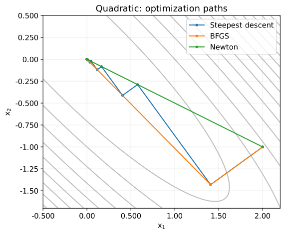
Start at $\mathbf{x}_0=(2,-1)^\top$ with $\mathbf{H}_0=\mathbf{I}$. In this experiment, we minimize exactly along each direction.
$$ \begin{aligned} \phi(\alpha)&=f(\mathbf{x}+\alpha\mathbf{p}),\\ \phi^{\prime}(\alpha)&=\mathbf{p}^\top\mathbf{A}\mathbf{x} +\alpha\mathbf{p}^\top\mathbf{A}\mathbf{p},\\ \phi^{\prime}(\alpha)=0&\Longrightarrow \alpha=-\frac{\mathbf{g}^\top\mathbf{p}}{\mathbf{p}^\top\mathbf{A}\mathbf{p}}. \end{aligned} $$
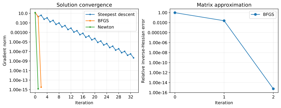
The step length using $\mathbf{A}$ is only for comparison on this known quadratic. For general functions, use the line search from the previous section. Steepest descent uses $\mathbf{p}=-\mathbf{g}$, while Newton’s method solves $\mathbf{A}\mathbf{p}=-\mathbf{g}$. Figure 2 shows the paths; Figure 3 shows the gradient norm and relative inverse-Hessian error.
A = np.array([[10, 9], [9, 10]], dtype=float)
x0 = np.array([2, -1], dtype=float)


def quadratic(x):
    return (x @ A @ x) / 2


def quadratic_grad(x):
    return A @ x


def exact_step(x, g, p):
    return -(g @ p) / (p @ A @ p)


quad = bfgs_trace(quadratic, quadratic_grad, x0, step=exact_step)
gd = [x0.copy()]
for _ in range(300):
    g = quadratic_grad(gd[-1])
    if np.linalg.norm(g) <= 1.00e-8:
        break
    p = -g
    gd.append(gd[-1] + exact_step(gd[-1], g, p) * p)

# For the Newton comparison, compute the direction using the true Hessian.
newton = np.array([x0, x0 - np.linalg.solve(A, quadratic_grad(x0))])
paths = {"Steepest descent": np.array(gd), "BFGS": quad["x"], "Newton": newton}
pprint({name: {"iterations": len(path) - 1,
               "gradient_norm": f"{np.linalg.norm(A @ path[-1]):#.3g}"}
        for name, path in paths.items()})

u, v = np.meshgrid(np.linspace(-0.500, 2.20, 200), np.linspace(-1.70, 0.500, 200))
fig, ax = plt.subplots(figsize=(6.80, 4.80), layout="constrained")
ax.contour(u, v, 5*u**2 + 9*u*v + 5*v**2, levels=15, colors="0.750")
for name, path in paths.items():
    ax.plot(path[:, 0], path[:, 1], "o-", markersize=3, label=name)
ax.set(xlabel="$x_1$", ylabel="$x_2$", title="Quadratic: optimization paths", aspect="equal")
save_figure(fig, "02_quadratic_path.svg")
{'BFGS': {'gradient_norm': '3.30e-15', 'iterations': 2},
 'Newton': {'gradient_norm': '1.49e-15', 'iterations': 1},
 'Steepest descent': {'gradient_norm': '4.58e-09', 'iterations': 33}}
true_inverse = np.linalg.solve(A, np.eye(2))
matrix_error = np.linalg.norm(quad["H"] - true_inverse, axis=(1, 2)) / np.linalg.norm(true_inverse)
fig, axes = plt.subplots(1, 2, figsize=(10, 3.80), layout="constrained")
for name, path in paths.items():
    # Apply a lower plotting bound for logarithmic axes.
    norm = np.linalg.norm(path @ A.T, axis=1)
    axes[0].semilogy(np.maximum(norm, 1.00e-16), "o-", markersize=3, label=name)
axes[0].set(xlabel="Iteration", ylabel="Gradient norm", title="Solution convergence")
axes[1].semilogy(np.maximum(matrix_error, 1.00e-16), "o-", label="BFGS")
axes[1].set(xlabel="Iteration", ylabel="Relative inverse-Hessian error", title="Matrix approximation")
save_figure(fig, "03_quadratic_errors.svg")

print("Final inverse Hessian approximation:")
pprint(quad["H"][-1])
print("True inverse for comparison:")
pprint(true_inverse)
Final inverse Hessian approximation:
array([[0.526, -0.474],
       [-0.474, 0.526]])
True inverse for comparison:
array([[0.526, -0.474],
       [-0.474, 0.526]])
From this starting point, BFGS reaches the tolerance in two steps and Newton’s method in one. The output also gives the steepest descent count. With exact line searches and exact arithmetic, BFGS reaches the solution of a positive definite quadratic in at most $n$ steps. This bound does not apply directly to general nonlinear functions or calculations with rounding error.
Reaching the solution does not reconstruct the whole matrix
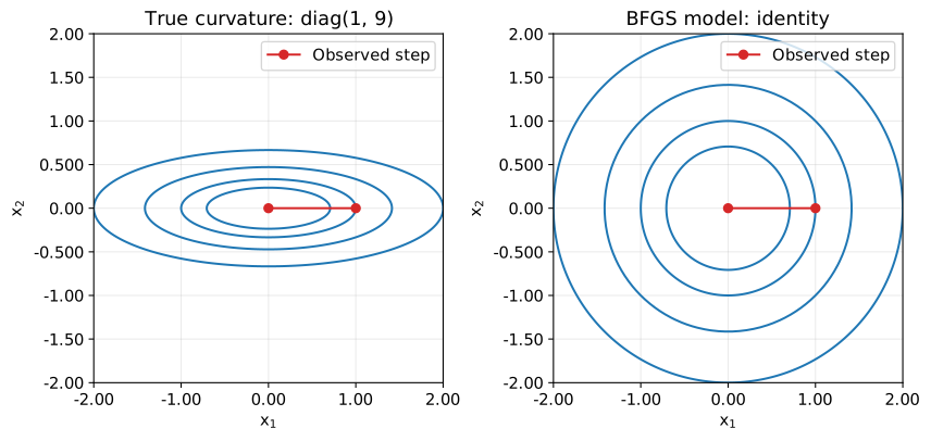
Let $\mathbf{D}=\operatorname{diag}(1,9)$ and $f(\mathbf{x})=\mathbf{x}^\top\mathbf{D}\mathbf{x}/2$, with $\mathbf{x}_0=(1,0)^\top$ and $\mathbf{H}_0=\mathbf{I}$.
$$ \begin{aligned} \mathbf{g}_0&=(1,0)^\top,\qquad \mathbf{p}_0=(-1,0)^\top,\\ \alpha_0&=1,\qquad \mathbf{x}_1=(0,0)^\top,\\ \mathbf{s}_0&=(-1,0)^\top,\qquad \mathbf{y}_0=(-1,0)^\top,\\ \rho_0&=1,\qquad \mathbf{v}_0=\mathbf{H}_0\mathbf{y}_0=\mathbf{s}_0,\\ \mathbf{H}_1&=\mathbf{I}+2\mathbf{s}_0\mathbf{s}_0^\top -2\mathbf{s}_0\mathbf{s}_0^\top=\mathbf{I} \ne\mathbf{D}^{-1}. \end{aligned} $$
The solution is reached without observing the curvature 9 in the second direction. Figure 4 compares the true quadratic with the model from the computed matrix, both centered at the optimum. They agree horizontally but not vertically.
D = np.diag([1, 9])
s = np.array([-1, 0], dtype=float)
partial_H, _ = inverse_bfgs(np.eye(2), s, D @ s)
pprint({"H_after_one_step": partial_H, "true_inverse": np.linalg.solve(D, np.eye(2))})
display(Math(r"\mathbf{H}_1=\begin{bmatrix}1&0\\0&1\end{bmatrix},"
             r"\qquad\mathbf{D}^{-1}=\begin{bmatrix}1&0\\0&1/9\end{bmatrix}"))

u, v = np.meshgrid(np.linspace(-2, 2, 200), np.linspace(-2, 2, 200))
fig, axes = plt.subplots(1, 2, figsize=(8.80, 4.20), layout="constrained")
for ax, z, title in zip(axes, [(u**2 + 9*v**2)/2, (u**2 + v**2)/2],
                        ["True curvature: diag(1, 9)", "BFGS model: identity"]):
    ax.contour(u, v, z, levels=[1/4, 1/2, 1, 2], colors="tab:blue")
    ax.plot([1, 0], [0, 0], "o-", color="tab:red", label="Observed step")
    ax.set(xlabel="$x_1$", ylabel="$x_2$", title=title, aspect="equal")
save_figure(fig, "04_unobserved_direction.svg")
{'H_after_one_step': array([[1.00, 0.00],
       [0.00, 1.00]]),
 'true_inverse': array([[1.00, 0.00],
       [0.00, 0.111]])}
$$ \displaystyle \mathbf{H}_1=\begin{bmatrix}1&0\\0&1\end{bmatrix},\qquad\mathbf{D}^{-1}=\begin{bmatrix}1&0\\0&1/9\end{bmatrix} $$
6. Testing a function with a changing Hessian
Use the Rosenbrock function. Its gradient follows from the chain rule.
$$ \begin{aligned} f(\mathbf{x})&=(1-x_1)^2+100(x_2-x_1^2)^2,\\ \frac{\partial f}{\partial x_1} &=-2(1-x_1)+200(x_2-x_1^2)(-2x_1)\\ &=2(x_1-1)-400x_1(x_2-x_1^2),\\ \frac{\partial f}{\partial x_2}&=200(x_2-x_1^2). \end{aligned} $$
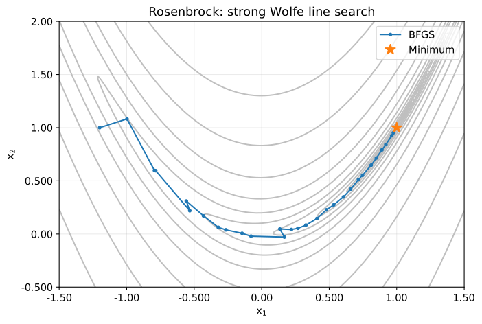
The minimizer is $\mathbf{x}_*=(1,1)^\top$. Start at $(-1.20,1.00)^\top$ and pass only function values and gradients to BFGS. Figure 5 shows the path along the narrow, curved valley.
def rosenbrock(x):
    return (1 - x[0])**2 + 100 * (x[1] - x[0]**2)**2


def rosenbrock_grad(x):
    a, b = x
    return np.array([2*(a - 1) - 400*a*(b - a**2), 200*(b - a**2)])


rosen = bfgs_trace(rosenbrock, rosenbrock_grad, [-1.20, 1.00])
pprint({"success": rosen["success"], "iterations": len(rosen["x"]) - 1,
        "x": rosen["x"][-1],
        "gradient_norm": f"{np.linalg.norm(rosenbrock_grad(rosen['x'][-1])):#.3g}",
        "skipped_updates": int(np.count_nonzero(~rosen["updated"]))})

u, v = np.meshgrid(np.linspace(-1.50, 1.50, 240), np.linspace(-0.500, 2, 240))
fig, ax = plt.subplots(figsize=(7.20, 4.80), layout="constrained")
ax.contour(u, v, (1-u)**2 + 100*(v-u**2)**2, levels=np.logspace(-2, 3, 14), colors="0.750")
ax.plot(rosen["x"][:, 0], rosen["x"][:, 1], "o-", markersize=3, label="BFGS")
ax.plot(1, 1, "*", markersize=12, label="Minimum")
ax.set(xlabel="$x_1$", ylabel="$x_2$", title="Rosenbrock: strong Wolfe line search")
save_figure(fig, "05_rosenbrock_path.svg")
{'gradient_norm': '2.87e-10',
 'iterations': 35,
 'skipped_updates': 0,
 'success': True,
 'x': array([1.00, 1.00])}
Compute the true Hessian only for checking the results. It is not supplied to the optimization procedure.
$$ \begin{aligned} \frac{\partial^2f}{\partial x_1^2} &=2-400(x_2-x_1^2)+800x_1^2=2-400x_2+1200x_1^2,\\ \frac{\partial^2f}{\partial x_2\partial x_1}&=-400x_1, \qquad \frac{\partial^2f}{\partial x_2^2}=200,\\ \nabla^2f(\mathbf{x}) &=\begin{bmatrix}2-400x_2+1200x_1^2&-400x_1\\-400x_1&200\end{bmatrix}. \end{aligned} $$
In Figure 6, use the Frobenius norm to measure the difference between $\mathbf{B}_k=\mathbf{H}_k^{-1}$ and the true Hessian at that point.
$$ e_k=\frac{\|\mathbf{B}_k-\nabla^2f(\mathbf{x}_k)\|_F} {\|\nabla^2f(\mathbf{x}_k)\|_F}, \qquad r_k=\frac{\|\mathbf{H}_{k+1}\mathbf{y}_k-\mathbf{s}_k\|_2}{\|\mathbf{s}_k\|_2}. $$
The gradient norm, full matrix error $e_k$, and secant residual $r_k$ measure different things. A small $r_k$ does not imply that $e_k$ is zero or decreases at every step. Since logarithmic axes cannot show zero, values in Figures 3 and 6 are clipped to $1.00\times10^{-16}$ for display only.
def rosenbrock_hessian(x):
    a, b = x
    return np.array([[2 - 400*b + 1200*a*a, -400*a], [-400*a, 200]])


grad_norm = np.array([np.linalg.norm(rosenbrock_grad(x)) for x in rosen["x"]])
errors = []
for x, H in zip(rosen["x"], rosen["H"]):
    B = np.linalg.solve(H, np.eye(2))  # Compute the inverse only for diagnostics.
    G = rosenbrock_hessian(x)
    errors.append(np.linalg.norm(B - G) / np.linalg.norm(G))

fig, axes = plt.subplots(3, 1, figsize=(8, 8.40), layout="constrained")
series = [(np.arange(len(grad_norm)), grad_norm, "Gradient norm"),
          (np.arange(len(errors)), errors, "Relative Hessian error"),
          (np.arange(1, len(rosen["x"])), rosen["residual"], "Relative secant residual")]
for ax, (indices, values, label) in zip(axes, series):
    ax.semilogy(indices, np.maximum(values, 1.00e-16), "o-", markersize=3)
    ax.set(xlabel="Iteration", ylabel=label)
save_figure(fig, "06_rosenbrock_diagnostics.svg")

# Check convergence and positive definiteness independently of the plots.
assert quad["success"] and rosen["success"]
assert np.linalg.norm(rosen["x"][-1] - np.ones(2)) < 1.00e-6
assert np.all(np.linalg.eigvalsh(rosen["H"]) > 0)
assert np.all(rosen["residual"][rosen["updated"]] < 1.00e-8)
pprint({"max_secant_residual": f"{np.max(rosen['residual']):#.3g}",
        "final_Hessian_error": f"{errors[-1]:#.3g}",
        "smallest_eigenvalue_of_H": f"{np.min(np.linalg.eigvalsh(rosen['H'])):#.3g}"})
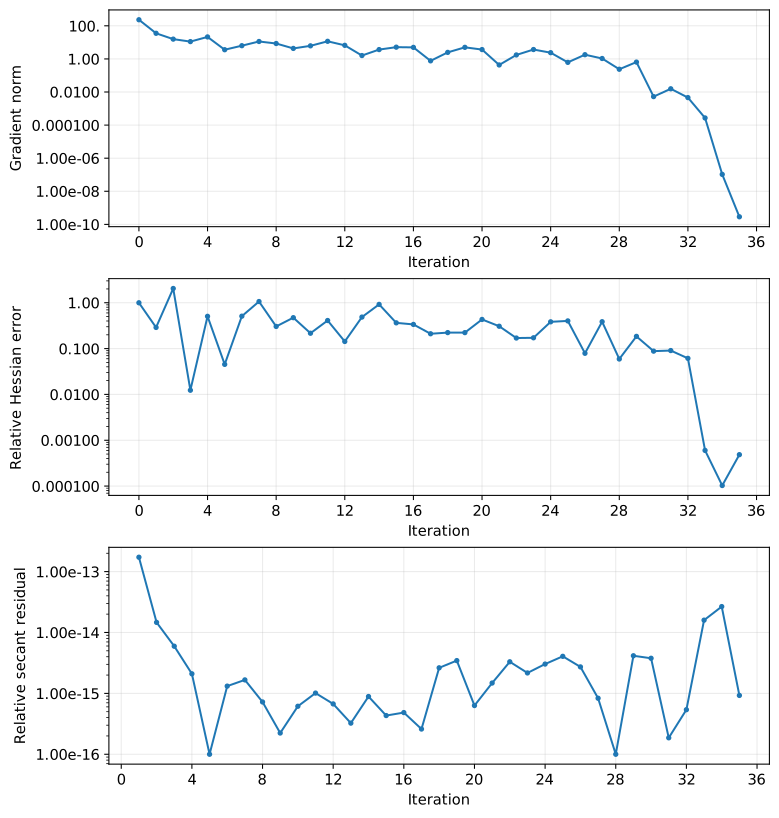
{'final_Hessian_error': '0.000484',
 'max_secant_residual': '1.72e-13',
 'smallest_eigenvalue_of_H': '0.000461'}
Running SciPy’s BFGS implementation
For practical use, pass method="BFGS" and the gradient jac to minimize. If the gradient is omitted, it is estimated by finite differences. “No Hessian required” therefore does not mean “no derivative information required.” See the SciPy documentation.
The returned hess_inv approximates the inverse Hessian. Details such as the line search differ from our implementation, so the iteration counts and final matrices need not match.
result = minimize(rosenbrock, [-1.20, 1.00], jac=rosenbrock_grad, method="BFGS",
                  options={"gtol": 1.00e-8, "norm": 2, "maxiter": 200})
pprint({"success": bool(result.success), "message": str(result.message),
        "iterations": int(result.nit), "x": result.x,
        "gradient_norm": f"{np.linalg.norm(result.jac):#.3g}",
        "hess_inv": result.hess_inv})
assert result.success
assert np.linalg.norm(result.x - rosen["x"][-1]) < 1.00e-6
{'gradient_norm': '1.62e-11',
 'hess_inv': array([[0.501, 1.00],
       [1.00, 2.01]]),
 'iterations': 34,
 'message': 'Optimization terminated successfully.',
 'success': True,
 'x': array([1.00, 1.00])}
Conclusion
We examined how BFGS uses steps and gradient differences to update a Hessian or inverse-Hessian approximation that determines the search direction.
The secant condition matches the matrix action in the observed direction. It does not imply recovery of every true Hessian entry or a decrease in matrix error at every step. Positive curvature and positive definiteness provide a descent direction; the line search chooses the step length.
BFGS avoids second derivatives and repeated matrix inversion, but stores a dense matrix using $O(n^2)$ memory. For many variables, L-BFGS is an option that keeps only a small number of steps and gradient differences.