What is a canonical link? (Rewritten from an earlier blog post)
Environment
Python 3.14.6, NumPy 2.5.4, SciPy 1.18.1, SymPy 1.14.0, Matplotlib 3.11.2 (Jupyter Notebook).
This article is a rewrite of a post from around 2013–2016, with calculations performed in the environment described above.
Overview
A canonical link connects the mean of a generalized linear model (GLM) to its natural parameter. We derive the formulas for normal, Bernoulli, and Poisson distributions, then use Python to examine the functions and fitted regression models.
Setup
Run the code in Jupyter Notebook from top to bottom. Round numbers to three significant digits only when displaying them.
import platform
from pathlib import Path
from pprint import pprint

import matplotlib
import matplotlib.pyplot as plt
import numpy as np
import scipy
import sympy as sp
from IPython.display import Latex, SVG, display
from matplotlib.ticker import FuncFormatter
from scipy.optimize import minimize
from scipy.special import expit, logit, ndtr

print(f"Python: {platform.python_version()}")
print(f"NumPy: {np.__version__}, SciPy: {scipy.__version__}")
print(f"SymPy: {sp.__version__}, Matplotlib: {matplotlib.__version__}")

output_dir = Path("101_nb_files")
output_dir.mkdir(exist_ok=True)


def sig3(value):
    """Display three significant digits, keeping trailing zeros."""
    return format(float(value), "#.3g")


np.set_printoptions(formatter={"float_kind": sig3})
plt.rcParams.update({"font.size": 11, "svg.fonttype": "none"})


def show_math(source):
    """Convert the delimiters of key formulas to $$ for display."""
    body = source.removeprefix(r"\(").removesuffix(r"\)")
    display(Latex("$$" + body + "$$"))


def save_figure(fig, name):
    """Format tick labels and display the saved SVG directly."""
    for ax in fig.axes:
        ax.xaxis.set_major_formatter(FuncFormatter(lambda v, _: sig3(v)))
        ax.yaxis.set_major_formatter(FuncFormatter(lambda v, _: sig3(v)))
        ax.grid(alpha=0.250)
    path = output_dir / name
    fig.savefig(path, format="svg", bbox_inches="tight")
    plt.close(fig)
    display(SVG(filename=str(path)))
Python: 3.14.6
NumPy: 2.5.4, SciPy: 1.18.1
SymPy: 1.14.0, Matplotlib: 3.11.2
1. Connecting the mean and the linear predictor
Let $\mathbf{x}_i$ be the explanatory variables and $\mathbf{w}$ the coefficients. Include an intercept by placing a 1 at the start of $\mathbf{x}_i$. The conditional mean $\mu_i$ and linear predictor $\eta_i$ are related by
$$ \mu_i=E[Y_i\mid\mathbf{x}_i],\qquad \eta_i=\mathbf{x}_i^{\mathsf T}\mathbf{w},\qquad g(\mu_i)=\eta_i $$
The link $g$ maps the mean to the linear predictor, and the inverse link $g^{-1}$ maps the predictor back to the mean. This does not mean transforming the response $Y_i$ itself and regressing the transformed values.
Write the conditional distribution in the following exponential-family form.
$$ f(y;\theta,\phi)=\exp\left\{\frac{y\theta-b(\theta)}{a(\phi)}+c(y,\phi)\right\}. $$
Here, $\theta$ is the natural parameter and $\phi$ is a parameter related to variance. Assume $a(\phi)>0$ and hold $\phi$ fixed when differentiating. If the support does not depend on $\theta$ and differentiation can be exchanged with integration, the fact that the density integrates to one gives
$$ \begin{aligned} 0&=\frac{\partial}{\partial\theta}\int f(y;\theta,\phi)\,dy\\ &=\int f(y;\theta,\phi)\frac{y-b^{\prime}(\theta)}{a(\phi)}\,dy =\frac{E[Y]-b^{\prime}(\theta)}{a(\phi)},\\ \mu&=b^{\prime}(\theta) \end{aligned} $$
For discrete distributions, replace integrals with sums. Choosing the inverse of $b^{\prime}$ as the link gives $\eta=\theta$. This defines the canonical link. The same definition appears in these GLM lecture notes.
show_math(r"\(\boxed{g_{\mathrm c}(\mu)=(b')^{-1}(\mu),\quad \eta=\theta}\)")
$$\boxed{g_{\mathrm c}(\mu)=(b^{\prime})^{-1}(\mu),\quad \eta=\theta}$$
2. Finding the canonical link from a distribution
Bernoulli: the logit link
If $Y\in\{0,1\}$ and $P(Y=1)=p$, then $\mu=p$. Rewrite the probability mass function in exponential-family form.
$$ \begin{aligned} P(Y=y)&=p^y(1-p)^{1-y}\\ &=\exp\{y\log p+(1-y)\log(1-p)\}\\ &=\exp\left\{y\log\frac{p}{1-p}+\log(1-p)\right\}. \end{aligned} $$
The coefficient of $y$ gives $\theta=\log\{p/(1-p)\}$. Solving for $p$ gives
$$ e^\theta=\frac{p}{1-p} \ \Rightarrow\ e^\theta(1-p)=p \ \Rightarrow\ e^\theta=p(1+e^\theta) \ \Rightarrow\ p=\frac{e^\theta}{1+e^\theta}. $$
Since $1-p=1/(1+e^\theta)$, we obtain $b(\theta)=-\log(1-p)=\log(1+e^\theta)$, $a=1$, and $c=0$.
$$ \mu=b^{\prime}(\theta)=\frac{e^\theta}{1+e^\theta},\qquad g_{\mathrm c}(\mu)=\log\frac{\mu}{1-\mu},\qquad g_{\mathrm c}^{-1}(\eta)=\frac{1}{1+e^{-\eta}}. $$
The mean lies in $0<\mu<1$. The logit maps it to a real-valued linear predictor, while the inverse link, the logistic function, maps the predictor back to a value between zero and one.
Poisson: the log link
The response $Y$ is a nonnegative integer, with mean $\lambda>0$.
$$ \begin{aligned} P(Y=y)&=\frac{\lambda^y e^{-\lambda}}{y!} =\exp\{y\log\lambda-\lambda-\log(y!)\},\\ \theta&=\log\lambda,\quad b(\theta)=e^\theta,\quad a=1,\quad c=-\log(y!),\\ \mu&=b^{\prime}(\theta)=e^\theta=\lambda,\\ g_{\mathrm c}(\mu)&=\log\mu,\qquad g_{\mathrm c}^{-1}(\eta)=e^\eta. \end{aligned} $$
Normal: the identity link
Expand the log density of $Y\sim N(\mu,\sigma^2)$.
$$ \begin{aligned} \log f(y)&=-\frac{(y-\mu)^2}{2\sigma^2}-\frac12\log(2\pi\sigma^2)\\ &=-\frac{y^2-2y\mu+\mu^2}{2\sigma^2}-\frac12\log(2\pi\sigma^2)\\ &=\frac{y\mu-\mu^2/2}{\sigma^2} -\frac{y^2}{2\sigma^2}-\frac12\log(2\pi\sigma^2). \end{aligned} $$
Setting $a=\sigma^2$ gives $\theta=\mu$ and $b(\theta)=\theta^2/2$, so $b^{\prime}(\theta)=\theta$. Therefore, $g_{\mathrm c}(\mu)=\mu$. Below, we differentiate the expressions for all three distributions symbolically.
theta = sp.Symbol("theta", real=True)
families = {
    "Normal": theta**2 / 2,
    "Bernoulli": sp.log(1 + sp.exp(theta)),
    "Poisson": sp.exp(theta),
}
for name, b in families.items():
    print(name)
    derivative = sp.diff(b, theta)
    show_math(r"\(b(\theta)=" + sp.latex(b)
              + r",\quad b'(\theta)=" + sp.latex(derivative) + r"\)")

# Check logit and log values numerically. Use pprint for array results.
probabilities = np.array([0.200, 0.500, 0.800])
pprint(logit(probabilities))
pprint(expit(logit(probabilities)))
show_math(r"\(\log\frac{0.800}{1-0.800}=\log 4\approx "
          + sig3(logit(0.800)) + r"\)")
show_math(r"\(\log 3\approx " + sig3(np.log(3)) + r",\quad e^{\log 3}=3\)")
Normal
$$b(\theta)=\frac{\theta^{2}}{2},\quad b^{\prime}(\theta)=\theta$$
Bernoulli
$$b(\theta)=\log{\left(e^{\theta} + 1 \right)},\quad b^{\prime}(\theta)=\frac{e^{\theta}}{e^{\theta} + 1}$$
Poisson
$$b(\theta)=e^{\theta},\quad b^{\prime}(\theta)=e^{\theta}$$
array([-1.39, 0.00, 1.39])
array([0.200, 0.500, 0.800])
$$\log\frac{0.800}{1-0.800}=\log 4\approx 1.39$$
$$\log 3\approx 1.10,\quad e^{\log 3}=3$$
3. Plotting links and inverse links
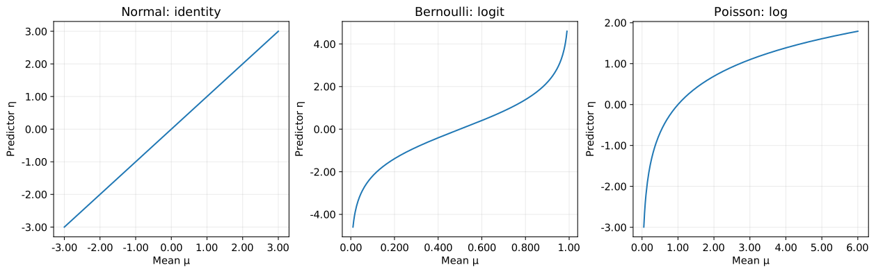
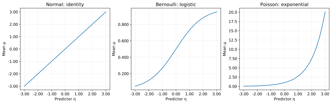
The first figure maps the mean to the predictor; the next shows the inverse mapping. The inverse link keeps the Bernoulli mean between zero and one and the Poisson mean positive. The normal mean has no such restriction.
# Use the mean domain appropriate to each distribution and avoid divergent endpoint values.
normal_mu = np.linspace(-3, 3, 300)
bernoulli_mu = np.linspace(0.0100, 0.990, 300)
poisson_mu = np.linspace(0.0500, 6, 300)
link_data = [
    (normal_mu, normal_mu, "Normal: identity"),
    (bernoulli_mu, logit(bernoulli_mu), "Bernoulli: logit"),
    (poisson_mu, np.log(poisson_mu), "Poisson: log"),
]
fig, axes = plt.subplots(1, 3, figsize=(13, 4), layout="constrained")
for ax, (mu, eta, title) in zip(axes, link_data):
    ax.plot(mu, eta)
    ax.set(xlabel=r"Mean $\mu$", ylabel=r"Predictor $\eta$", title=title)
save_figure(fig, "canonical_links.svg")

eta_grid = np.linspace(-3, 3, 300)
inverse_data = [
    (eta_grid, "Normal: identity"),
    (expit(eta_grid), "Bernoulli: logistic"),
    (np.exp(eta_grid), "Poisson: exponential"),
]
fig, axes = plt.subplots(1, 3, figsize=(13, 4), layout="constrained")
for ax, (mu, title) in zip(axes, inverse_data):
    ax.plot(eta_grid, mu)
    ax.set(xlabel=r"Predictor $\eta$", ylabel=r"Mean $\mu$", title=title)
save_figure(fig, "inverse_links.svg")
4. Why the estimation formulas become simpler
Consider independent observations with a common $a=a(\phi)$. With a canonical link, $\theta_i=\eta_i$, so differentiating the log-likelihood with respect to the coefficients gives
$$ \begin{aligned} \ell(\mathbf{w})&=\sum_i\left\{\frac{y_i\eta_i-b(\eta_i)}{a}+c(y_i,\phi)\right\},\\ \frac{\partial\ell}{\partial w_j} &=\sum_i\frac{y_i-b^{\prime}(\eta_i)}{a}\frac{\partial\eta_i}{\partial w_j} =\frac1a\sum_i(y_i-\mu_i)x_{ij}. \end{aligned} $$
Furthermore, $\partial\mu_i/\partial w_k=b^{\prime\prime}(\eta_i)x_{ik}$ gives the following for the negative log-likelihood $L=-\ell$.
$$ \nabla L=\frac1a\mathbf{X}^{\mathsf T}(\mathbf{m}-\mathbf{y}),\qquad \frac{\partial^2 L}{\partial w_j\partial w_k} =\frac1a\sum_i b^{\prime\prime}(\eta_i)x_{ij}x_{ik} $$
Each row of $\mathbf{X}$ is $\mathbf{x}_i^{\mathsf T}$, and the entries of $\mathbf{m}$ are $\mu_i$. For the Bernoulli distribution, the second derivative is
$$ b^{\prime\prime}(\eta)=\frac{e^\eta(1+e^\eta)-e^{2\eta}}{(1+e^\eta)^2} =\frac{e^\eta}{1+e^\eta}\frac1{1+e^\eta}=\mu(1-\mu) $$
For the Poisson distribution, $b^{\prime\prime}(\eta)=e^\eta=\mu$.
The following maximum-likelihood calculation uses this gradient and Hessian. We consider the two distributions with $a=1$, omitting terms that do not depend on the coefficients. In the numerical calculation, we divide the objective and its derivatives by the number of observations; this does not change the minimum. Generate 400 observations with a fixed random seed.
def fit_glm(X, y, family):
    """Fit a Bernoulli or Poisson model by maximum likelihood with its canonical link."""
    def terms(w):
        eta = X @ w
        if family == "Bernoulli":
            # Compute log(1 + exp(eta)) in a form that avoids overflow.
            mu = expit(eta)
            b = np.logaddexp(0, eta)
            variance = mu * (1 - mu)
        elif family == "Poisson":
            mu = np.exp(eta)
            b = mu
            variance = mu
        else:
            raise ValueError("Unsupported distribution")
        return eta, mu, b, variance

    def objective(w):
        eta, _, b, _ = terms(w)
        return np.mean(b - y * eta)

    def gradient(w):
        _, mu, _, _ = terms(w)
        return X.T @ (mu - y) / y.size

    def hessian(w):
        _, _, _, variance = terms(w)
        return X.T @ (variance[:, None] * X) / y.size

    result = minimize(
        objective, np.zeros(X.shape[1]), jac=gradient, hess=hessian,
        method="trust-exact", options={"gtol": 1.00e-8},
    )
    if not result.success:
        raise RuntimeError(result.message)
    return result


rng = np.random.default_rng(101)
x = np.linspace(-2, 2, 400)
X = np.column_stack([np.ones(x.size), x])
settings = [
    ("Bernoulli", np.array([-0.400, 1.20]), expit, "bernoulli_fit.svg"),
    ("Poisson", np.array([0.300, 0.650]), np.exp, "poisson_fit.svg"),
]
fit_results = {}
for family, w_true, inverse_link, filename in settings:
    mu_true = inverse_link(X @ w_true)
    y = (rng.binomial(1, mu_true) if family == "Bernoulli"
         else rng.poisson(mu_true))
    result = fit_glm(X, y, family)
    fit_results[family] = result
    print(f"{family}: coefficients are [intercept, slope]")
    pprint({"true coefficients": w_true, "estimated coefficients": result.x})
    pprint({"converged": bool(result.success), "iterations": int(result.nit),
            "maximum absolute mean gradient": sig3(np.max(np.abs(result.jac)))})

    fig, ax = plt.subplots(figsize=(7, 4), layout="constrained")
    ax.scatter(x, y, s=12, alpha=0.250, label="Observed")
    ax.plot(x, mu_true, color="black", linestyle="--", label="True mean")
    ax.plot(x, inverse_link(X @ result.x), color="tab:red", label="Fitted mean")
    ax.set(xlabel="x", ylabel="y / mean", title=f"{family}: canonical link")
    ax.legend()
    save_figure(fig, filename)
Bernoulli: coefficients are [intercept, slope]
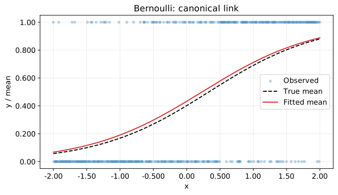
{'estimated coefficients': array([-0.271, 1.17]), 'true coefficients': array([-0.400, 1.20])}
{'iterations': 5, 'converged': True, 'maximum absolute mean gradient': '3.82e-16'}
Poisson: coefficients are [intercept, slope]
{'estimated coefficients': array([0.290, 0.640]), 'true coefficients': array([0.300, 0.650])}
{'iterations': 5, 'converged': True, 'maximum absolute mean gradient': '6.33e-10'}
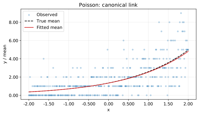
The fitted curves describe conditional means, not curves that pass through every observation. Because the random samples are finite, the estimated coefficients differ from those used to generate the data.
5. Other links are also possible
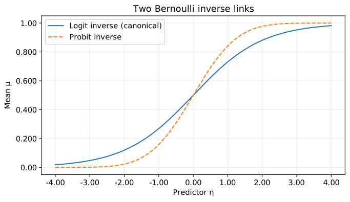
A Bernoulli model can also use the probit link $g(\mu)=\Phi^{-1}(\mu)$. Here, $\Phi$ is the standard normal cumulative distribution function, and the inverse link is $\Phi(\eta)$. A link can restrict the mean to the same range without making the linear predictor equal to the natural parameter.
The next plot compares the two inverse links at the same $\eta$. It does not compare the predictive accuracy of fitted models. A canonical link is convenient for calculation, but it does not always give better predictions. The choice of link should also reflect the relation between the mean and the explanatory variables.
eta = np.linspace(-4, 4, 400)
fig, ax = plt.subplots(figsize=(7, 4), layout="constrained")
ax.plot(eta, expit(eta), label="Logit inverse (canonical)")
ax.plot(eta, ndtr(eta), linestyle="--", label="Probit inverse")
ax.set(xlabel=r"Predictor $\eta$", ylabel=r"Mean $\mu$", title="Two Bernoulli inverse links")
ax.legend()
save_figure(fig, "link_comparison.svg")
Conclusion
We derived canonical links from the relation between the mean and natural parameter, examined three common distributions, and fitted example models in Python.
The canonical link is $g_{\mathrm c}=(b^{\prime})^{-1}$, making the linear predictor equal to the natural parameter. It is the identity for a normal distribution, the logit for a Bernoulli distribution, and the logarithm for a Poisson distribution. It simplifies likelihood derivatives, but whether it suits the data is a separate question.