Deriving GLMs from the exponential family (Rewritten from an earlier blog post)
Environment
Python 3.14.6, NumPy 2.5.4, SciPy 1.18.1, SymPy 1.14.0, Matplotlib 3.11.2 (Jupyter Notebook).
This article is a rewrite of a post from around 2013–2016, with calculations performed in the environment described above.
Overview
We derive generalized linear models (GLMs) from the exponential family. Writing normal, Bernoulli, and Poisson distributions in a common form connects maximum likelihood to iteratively reweighted least squares (IRLS). Finally, we fit a Poisson regression to artificial data.
Setup
Run the code in Jupyter Notebook from top to bottom. Round numbers to three significant digits only when displaying them.
import platform
from pathlib import Path
from pprint import pprint

import matplotlib
import matplotlib.pyplot as plt
from matplotlib.ticker import FuncFormatter, MaxNLocator
import numpy as np
import scipy
from scipy.optimize import minimize
from scipy.special import expit, gammaln
from scipy.stats import bernoulli, norm, poisson
import sympy as sp
from IPython.display import Latex, SVG, display

print(f'Python: {platform.python_version()}')
for name, module in [('NumPy', np), ('SciPy', scipy),
                     ('Matplotlib', matplotlib), ('SymPy', sp)]:
    print(f'{name}: {module.__version__}')

image_dir = Path('102_nb_files')
image_dir.mkdir(exist_ok=True)

# Keep full calculation precision and round to three significant digits only for output.
def sig3(value):
    text = f'{float(value):#.3g}'
    return text[:-1] if text.endswith('.') else text


np.set_printoptions(formatter={'float_kind': sig3})
plt.rcParams.update({
    'font.family': 'DejaVu Sans',
    'font.size': 11,
    'axes.spines.top': False,
    'axes.spines.right': False,
    'svg.fonttype': 'path',
})


def save_svg(fig, filename):
    # Also use three significant digits for decimal tick labels; save and display the SVG.
    for ax in fig.axes:
        ax.xaxis.set_major_formatter(FuncFormatter(lambda x, _: sig3(x)))
        ax.yaxis.set_major_formatter(FuncFormatter(lambda y, _: sig3(y)))
        ax.grid(alpha=0.200)
    path = image_dir / filename
    fig.savefig(path, format='svg', bbox_inches='tight')
    plt.close(fig)
    display(SVG(filename=str(path)))
Python: 3.14.6
NumPy: 2.5.4
SciPy: 1.18.1
Matplotlib: 3.11.2
SymPy: 1.14.0
1. Obtaining the mean and variance from normalization
We consider exponential-family distributions in which the response $y$ appears in the following form. Here, $\theta$ is the natural parameter, $\phi>0$ the dispersion parameter, and $b$ the function that provides normalization.
$$ f(y;\theta,\phi)=\exp\left\{\frac{y\theta-b(\theta)}{\phi}+c(y,\phi)\right\}. $$
Hold $\phi$ fixed. Assume the support does not depend on $\theta$ and that differentiation can be exchanged with integration. For discrete distributions, replace integrals with sums. First, differentiate the normalization condition once.
$$ \begin{aligned} \int f(y;\theta,\phi)\,dy&=1,\\ \frac{\partial f}{\partial\theta}&=f\frac{y-b^{\prime}(\theta)}{\phi},\\ 0=\int\frac{\partial f}{\partial\theta}\,dy &=\frac{E[Y]-b^{\prime}(\theta)}{\phi}. \end{aligned} $$
Thus, $\mu=E[Y]=b^{\prime}(\theta)$. Differentiating once more gives
$$ \begin{aligned} \frac{\partial^2 f}{\partial\theta^2} &=f\left\{\frac{(y-b^{\prime}(\theta))^2}{\phi^2}-\frac{b^{\prime\prime}(\theta)}{\phi}\right\},\\ 0=\int\frac{\partial^2 f}{\partial\theta^2}\,dy &=\frac{E[(Y-\mu)^2]}{\phi^2}-\frac{b^{\prime\prime}(\theta)}{\phi},\\ \operatorname{Var}(Y)&=\phi b^{\prime\prime}(\theta). \end{aligned} $$
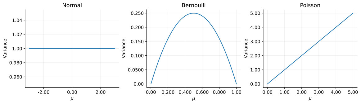
The mean is the first derivative of $b$, and the variance is the second derivative multiplied by $\phi$. Substituting the appropriate $b$ for each distribution gives its mean and variance by the same procedure.
# Also display the key relation as LaTeX output.
display(Latex(r'\(\displaystyle \mu=b^{\prime}(\theta),\qquad '
              r'\operatorname{Var}(Y)=\phi b^{\prime\prime}(\theta)\)'))

# Differentiate b symbolically for three distributions to check the mean and variance / phi.
theta = sp.Symbol('theta', real=True)
cumulants = {
    'Normal': theta**2 / 2,
    'Bernoulli': sp.log(1 + sp.exp(theta)),
    'Poisson': sp.exp(theta),
}
for name, b in cumulants.items():
    first = sp.diff(b, theta)
    second = sp.simplify(sp.diff(first, theta))
    print(name)
    display(Latex(
        r'\(\displaystyle b(\theta)=' + sp.latex(b)
        + r',\quad b^{\prime}(\theta)=' + sp.latex(first)
        + r',\quad b^{\prime\prime}(\theta)=' + sp.latex(second) + r'\)'
    ))
$$ \displaystyle \mu=b^{\prime}(\theta),\qquad \operatorname{Var}(Y)=\phi b^{\prime\prime}(\theta) $$
Normal
$$ \displaystyle b(\theta)=\frac{\theta^{2}}{2},\quad b^{\prime}(\theta)=\theta,\quad b^{\prime\prime}(\theta)=1 $$
Bernoulli
$$ \displaystyle b(\theta)=\log{\left(e^{\theta} + 1 \right)},\quad b^{\prime}(\theta)=\frac{e^{\theta}}{e^{\theta} + 1},\quad b^{\prime\prime}(\theta)=\frac{e^{\theta}}{e^{2 \theta} + 2 e^{\theta} + 1} $$
Poisson
$$ \displaystyle b(\theta)=e^{\theta},\quad b^{\prime}(\theta)=e^{\theta},\quad b^{\prime\prime}(\theta)=e^{\theta} $$
2. Rewriting three distributions
For the normal distribution $N(\mu,\sigma^2)$, expand the square.
$$ \begin{aligned} \log f(y)&=-\frac{(y-\mu)^2}{2\sigma^2}-\frac12\log(2\pi\sigma^2)\\ &=\frac{y\mu-\mu^2/2}{\sigma^2}-\frac{y^2}{2\sigma^2}-\frac12\log(2\pi\sigma^2). \end{aligned} $$
For the Bernoulli distribution, $y\in\{0,1\}$ and $0<p<1$. Setting $\theta=\log\{p/(1-p)\}$ gives $p=e^\theta/(1+e^\theta)$.
$$ \begin{aligned} \log f(y)&=y\log p+(1-y)\log(1-p)\\ &=y\log\frac{p}{1-p}+\log(1-p)\\ &=y\theta-\log(1+e^\theta). \end{aligned} $$
For the Poisson distribution, $y=0,1,\ldots$ and $\lambda>0$. Set $\theta=\log\lambda$.
$$ \begin{aligned} f(y)&=\frac{e^{-\lambda}\lambda^y}{y!},\\ \log f(y)&=y\log\lambda-\lambda-\log(y!)\\ &=y\theta-e^\theta-\log(y!). \end{aligned} $$
Comparing each expression with the general form gives the following table. The term $c$ is the part of each expression outside $\{y\theta-b(\theta)\}/\phi$.
| Distribution | $\theta$ | $b(\theta)$ | $\phi$ | $\mu$ | Variance |
|---|---|---|---|---|---|
| Normal | $\mu$ | $\theta^2/2$ | $\sigma^2$ | $\theta$ | $\sigma^2$ |
| Bernoulli | $\log\{p/(1-p)\}$ | $\log(1+e^\theta)$ | $1$ | $p$ | $p(1-p)$ |
| Poisson | $\log\lambda$ | $e^\theta$ | $1$ | $\lambda$ | $\lambda$ |
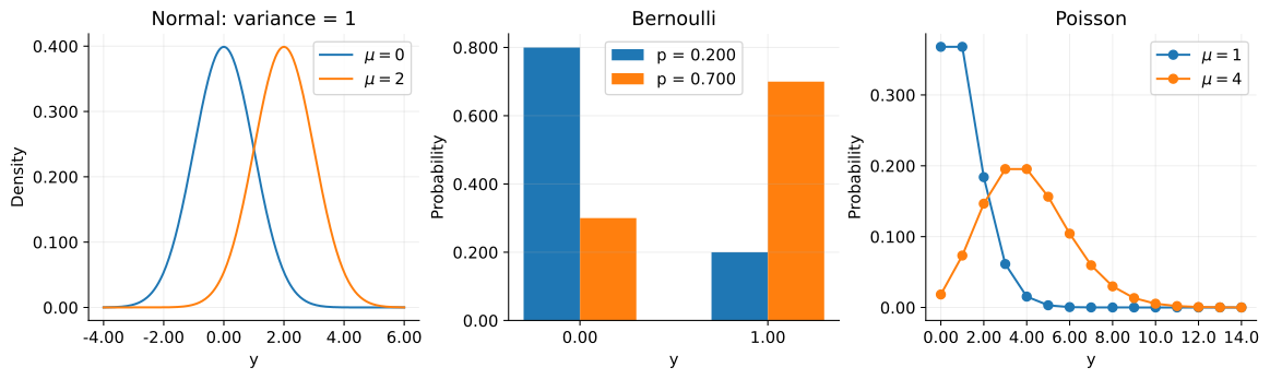
The normal distribution models continuous values, the Bernoulli distribution binary values, and the Poisson distribution nonnegative integers.
fig, axes = plt.subplots(1, 3, figsize=(12, 3.50), layout='constrained')
grid = np.linspace(-4, 6, 400)
for mu in (0, 2):
    axes[0].plot(grid, norm.pdf(grid, loc=mu), label=rf'$\mu={mu}$')
axes[0].set(title='Normal: variance = 1', xlabel='y', ylabel='Density')

for p, shift in ((0.200, -0.150), (0.700, 0.150)):
    axes[1].bar(np.array([0, 1]) + shift, bernoulli.pmf([0, 1], p),
                width=0.300, label=f'p = {sig3(p)}')
axes[1].set(title='Bernoulli', xlabel='y', ylabel='Probability', xticks=[0, 1])

counts = np.arange(15)
for mu in (1, 4):
    axes[2].plot(counts, poisson.pmf(counts, mu), 'o-', label=rf'$\mu={mu}$')
axes[2].set(title='Poisson', xlabel='y', ylabel='Probability')
axes[2].xaxis.set_major_locator(MaxNLocator(integer=True))
for ax in axes:
    ax.legend()
save_svg(fig, '01_distributions.svg')
3. Connecting the mean to explanatory variables
Assume the observations $Y_i$ are independent conditional on the explanatory variables $\mathbf{x}_i$, and define $\mu_i=E[Y_i\mid\mathbf{x}_i]$. A GLM chooses a link function $g$ to connect the mean to a linear predictor.
$$ \eta_i=\mathbf{x}_i^{\mathsf T}\mathbf{\boldsymbol{\beta}},\qquad g(\mu_i)=\eta_i. $$
Include a $1$ in $\mathbf{x}_i$ for the intercept. The linear predictor and choice of link are model assumptions added to the distributional properties. They are not uniquely determined by the exponential family alone.
Where $b^{\prime\prime}>0$, we have $\theta_i=(b^{\prime})^{-1}(\mu_i)$. The choice $\eta_i=\theta_i$ is called a canonical link.
$$ g(\mu)=(b^{\prime})^{-1}(\mu),\qquad \mu_i=b^{\prime}(\eta_i). $$
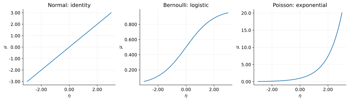
This gives the identity link $g(\mu)=\mu$ for the normal distribution, the logit link $g(\mu)=\log\{\mu/(1-\mu)\}$ for Bernoulli, and the log link $g(\mu)=\log\mu$ for Poisson.
eta = np.linspace(-3, 3, 300)
inverse_links = [eta, expit(eta), np.exp(eta)]
titles = ['Normal: identity', 'Bernoulli: logistic', 'Poisson: exponential']
fig, axes = plt.subplots(1, 3, figsize=(12, 3.40), layout='constrained')
for ax, mean, title in zip(axes, inverse_links, titles):
    ax.plot(eta, mean)
    ax.set(title=title, xlabel=r'$\eta$', ylabel=r'$\mu$')
save_svg(fig, '02_inverse_links.svg')

# Conditional variance as the conditional mean varies. Use phi = 1 for the normal distribution.
mean_grids = [np.linspace(-3, 3, 200), np.linspace(0, 1, 200),
              np.linspace(0, 5, 200)]
variances = [np.ones(200), mean_grids[1] * (1 - mean_grids[1]), mean_grids[2]]
fig, axes = plt.subplots(1, 3, figsize=(12, 3.40), layout='constrained')
for ax, mean, variance, title in zip(axes, mean_grids, variances, titles):
    ax.plot(mean, variance)
    ax.set(title=title.split(':')[0], xlabel=r'$\mu$', ylabel='Variance')
save_svg(fig, '03_mean_variance.svg')
4. From maximum likelihood to IRLS
From here on, hold the common $\phi$ fixed and use a canonical link. Differentiating the log-likelihood with the chain rule gives
$$ \begin{aligned} \ell(\mathbf{\boldsymbol{\beta}})&=\sum_i\left\{\frac{y_i\theta_i-b(\theta_i)}{\phi}+c(y_i,\phi)\right\},\\ \frac{\partial\ell}{\partial\beta_j} &=\sum_i\frac{y_i-b^{\prime}(\theta_i)}{\phi}\frac{\partial\theta_i}{\partial\beta_j} =\sum_i\frac{(y_i-\mu_i)x_{ij}}{\phi},\\ \frac{\partial\mu_i}{\partial\beta_k}&=b^{\prime\prime}(\eta_i)x_{ik},\\ \frac{\partial^2\ell}{\partial\beta_j\partial\beta_k} &=-\sum_i\frac{b^{\prime\prime}(\eta_i)x_{ij}x_{ik}}{\phi}. \end{aligned} $$
Let row $i$ of $\mathbf{X}$ be $\mathbf{x}_i^{\mathsf T}$, and set $\mathbf{W}=\operatorname{diag}\{b^{\prime\prime}(\eta_i)/\phi\}$. The gradient $\mathbf{U}$ and Hessian $\mathbf{H}$ are
$$ \mathbf{U}=\mathbf{X}^{\mathsf T}(\mathbf{y}-\mathbf{\boldsymbol{\mu}})/\phi, \qquad \mathbf{H}=-\mathbf{X}^{\mathsf T}\mathbf{W}\mathbf{X}. $$
The Newton update is $\mathbf{\boldsymbol{\beta}}_{\rm new}=\mathbf{\boldsymbol{\beta}}-\mathbf{H}^{-1}\mathbf{U}$. Introducing a working response $z_i$ gives
$$ \begin{aligned} z_i&=\eta_i+\frac{y_i-\mu_i}{b^{\prime\prime}(\eta_i)},\\ \mathbf{W}(\mathbf{z}-\mathbf{X}\mathbf{\boldsymbol{\beta}})&=(\mathbf{y}-\mathbf{\boldsymbol{\mu}})/\phi,\\ \mathbf{\boldsymbol{\beta}}_{\rm new} &=\mathbf{\boldsymbol{\beta}}+(\mathbf{X}^{\mathsf T}\mathbf{W}\mathbf{X})^{-1}\mathbf{U}\\ &=(\mathbf{X}^{\mathsf T}\mathbf{W}\mathbf{X})^{-1}\mathbf{X}^{\mathsf T}\mathbf{W}\mathbf{z}. \end{aligned} $$
This equation minimizes $\sum_i W_{ii}(z_i-\mathbf{x}_i^{\mathsf T}\mathbf{\boldsymbol{\beta}}_{\rm new})^2$. Recomputing the weights and working response from the mean at every step gives IRLS. The inverse exists when the columns of $\mathbf{X}$ are linearly independent and the weights are positive. The implementation does not compute the inverse directly.
5. Implementing Poisson regression
Since $\mu_i=\exp(\beta_0+\beta_1x_i)$, we have $b^{\prime\prime}(\eta_i)=\mu_i$ and $\phi=1$. Therefore, $W_{ii}=\mu_i$ and $z_i=\eta_i+(y_i-\mu_i)/\mu_i$. Generate 240 observations with true coefficients $(0.300,0.700)$ and a fixed random seed.
rng = np.random.default_rng(102)
x = np.linspace(-2, 2, 240)
X = np.column_stack([np.ones_like(x), x])
beta_true = np.array([0.300, 0.700])
mu_true = np.exp(X @ beta_true)
y = rng.poisson(mu_true)


def poisson_nll(beta):
    # Negative log-likelihood. Compute log(y!) with gammaln(y + 1).
    eta_now = X @ beta
    return np.sum(np.exp(eta_now) - y * eta_now + gammaln(y + 1))


def fit_poisson_irls(X, y, max_iter=50, tol=1.00e-10):
    # Set the initial mean to the sample mean, which is positive in this example.
    beta = np.array([np.log(y.mean()), 0])
    history = [beta.copy()]
    for _ in range(max_iter):
        eta_now = X @ beta
        mu = np.exp(eta_now)
        z = eta_now + (y - mu) / mu
        sqrt_w = np.sqrt(mu)

        # Solve least squares after scaling by sqrt(W); there is no need to form the weight matrix.
        beta_new = np.linalg.lstsq(
            X * sqrt_w[:, None], z * sqrt_w, rcond=None,
        )[0]
        history.append(beta_new.copy())
        if np.linalg.norm(beta_new - beta) < tol:
            return beta_new, np.asarray(history)
        beta = beta_new
    raise RuntimeError('IRLS did not converge within the iteration limit')


beta_hat, history = fit_poisson_irls(X, y)
mu_hat = np.exp(X @ beta_hat)

# Independently check the result by minimizing the derived negative log-likelihood with SciPy.
check = minimize(
    poisson_nll, np.zeros(2), method='trust-exact',
    jac=lambda beta: X.T @ (np.exp(X @ beta) - y),
    hess=lambda beta: X.T @ (np.exp(X @ beta)[:, None] * X),
    options={'gtol': 1.00e-8},
)
assert check.success, check.message
np.testing.assert_allclose(beta_hat, check.x, rtol=1.00e-7, atol=1.00e-9)
score = X.T @ (y - mu_hat)
assert np.linalg.norm(score, ord=np.inf) < 1.00e-7

pprint({'true coefficients': beta_true, 'IRLS': beta_hat, 'SciPy': check.x})
pprint({'iterations': len(history) - 1,
        'negative log-likelihood': sig3(poisson_nll(beta_hat)),
        'maximum absolute gradient': f'{np.max(np.abs(score)):.2e}',
        'maximum coefficient difference': f'{np.max(np.abs(beta_hat - check.x)):.2e}'})
display(Latex(
    r'\(\displaystyle \widehat{\mu}(x)=\exp('
    + sig3(beta_hat[0]) + '+' + sig3(beta_hat[1]) + r'x)\)'
))
{'IRLS': array([0.332, 0.782]),
 'SciPy': array([0.332, 0.782]),
 'true coefficients': array([0.300, 0.700])}
{'maximum coefficient difference': '2.38e-14', 'maximum absolute gradient': '2.21e-13', 'iterations': 6, 'negative log-likelihood': '365'}
$$ \displaystyle \widehat{\mu}(x)=\exp(0.332+0.782x) $$
fig, axes = plt.subplots(1, 2, figsize=(11, 3.80), layout='constrained')
axes[0].scatter(x, y, s=15, alpha=0.400, label='Observed')
axes[0].plot(x, mu_true, '--', color='black', label='True mean')
axes[0].plot(x, mu_hat, color='tab:red', label='Fitted mean')
axes[0].set(title='Poisson regression', xlabel='x', ylabel='Count / mean')
axes[0].legend()

# Pearson residuals divide each residual by the standard deviation specified by the distribution.
pearson = (y - mu_hat) / np.sqrt(mu_hat)
axes[1].scatter(mu_hat, pearson, s=15, alpha=0.500)
axes[1].axhline(0, color='black', linewidth=1)
axes[1].set(title='Pearson residuals', xlabel='Fitted mean', ylabel='Residual')
save_svg(fig, '04_poisson_fit.svg')

iterations = np.arange(len(history))
losses = np.array([poisson_nll(beta) for beta in history])
fig, axes = plt.subplots(1, 2, figsize=(11, 3.50), layout='constrained')
axes[0].plot(iterations, losses, 'o-')
axes[0].set(title='IRLS convergence', xlabel='Iteration', ylabel='Negative log-likelihood')
for j in range(2):
    axes[1].plot(iterations, history[:, j], 'o-', label=rf'$\beta_{j}$')
    axes[1].axhline(beta_true[j], linestyle='--', color=f'C{j}', alpha=0.600)
axes[1].set(title='Coefficients (dashed: true)', xlabel='Iteration', ylabel='Coefficient')
axes[1].legend()
for ax in axes:
    ax.xaxis.set_major_locator(MaxNLocator(integer=True))
save_svg(fig, '05_irls_convergence.svg')
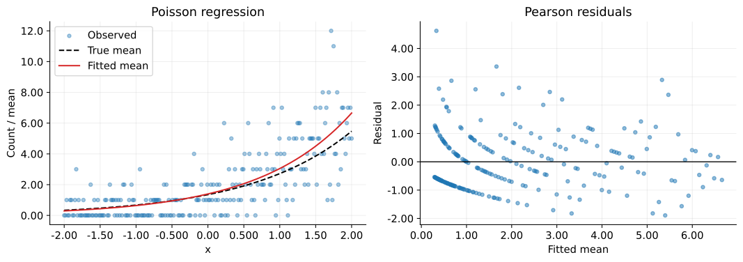
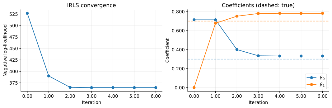
The solid line shows the estimated conditional mean; individual observations do not have to lie on it. Residuals are divided by $\sqrt{\widehat{\mu}_i}$. With a finite sample, estimated coefficients differ from the true ones. Agreement between IRLS and SciPy checks the calculation.
IRLS is not guaranteed to converge in every case. A Poisson distribution has equal conditional mean and variance. If real data have a larger variance, the choice of distribution should also be reconsidered.
Conclusion
We obtained the mean and variance by differentiating the exponential-family form and derived IRLS for fitting a GLM with a canonical link.
A GLM is specified by the response distribution, linear predictor, and link function. In this framework, normal, Bernoulli, and Poisson distributions lead to linear, logistic, and Poisson regression.