What do graph Laplacian eigenvalues mean? (Rewritten from an earlier blog post)
Environment
Python 3.14.6, NumPy 2.5.4, SciPy 1.18.1, SymPy 1.14.0, NetworkX 3.7, Matplotlib 3.11.2 (Jupyter Notebook).
This article is a rewrite of a post from around 2013–2016, with calculations performed in the environment described above.
Overview
Graph Laplacian eigenvalues describe variation in vertex values across edges. The number of zero eigenvalues gives the number of connected components, while the second eigenvalue relates to slow diffusion. We present the definitions and calculations and check them on small graphs.
Setup
Run the code in Jupyter Notebook from top to bottom. Round numbers to three significant digits only when displaying them.
import platform
from importlib.metadata import version
from pathlib import Path
from pprint import pprint

import matplotlib.pyplot as plt
import networkx as nx
import numpy as np
import sympy as sp
from IPython.display import Latex, SVG, display
from matplotlib.ticker import FuncFormatter, MaxNLocator
from scipy.linalg import eigh, expm

print(f"Python: {platform.python_version()}")
for package in ("numpy", "scipy", "matplotlib", "networkx", "sympy"):
    print(f"{package}: {version(package)}")

OUT = Path("101_nb_files")
OUT.mkdir(exist_ok=True)
plt.rcParams.update({"font.size": 11, "svg.fonttype": "path"})


def sig3(value):
    """Format nonzero decimals with three significant digits, including trailing zeros."""
    return "0" if value == 0 else f"{float(value):#.3g}"


np.set_printoptions(formatter={"float_kind": sig3})
tick_format = FuncFormatter(lambda value, _: sig3(value))


def laplacian(graph):
    # Use the same vertex order in the matrix and the graph.
    adjacency = nx.to_numpy_array(graph, nodelist=sorted(graph), weight="weight")
    degree = np.diag(adjacency.sum(axis=1))
    return degree - adjacency


def spectrum(matrix):
    # Use eigh for real symmetric matrices; it returns eigenvalues in ascending order.
    values, vectors = eigh(matrix)
    tolerance = 100 * np.finfo(float).eps * max(1, np.linalg.norm(matrix, 2))
    return values, vectors, tolerance


def show_figure(fig, name):
    path = OUT / f"{name}.svg"
    fig.savefig(path, format="svg", bbox_inches="tight")
    display(SVG(filename=str(path)))
    plt.close(fig)
Python: 3.14.6
numpy: 2.5.4
scipy: 1.18.1
matplotlib: 3.11.2
networkx: 3.7
sympy: 1.14.0
1. Definition
Consider an undirected graph without self-loops. Let the number of vertices be $n\geq2$ and the edge weights satisfy $w_{ij}=w_{ji}\geq0$, with zero weight meaning no edge. Define the adjacency matrix $\mathbf{A}=(w_{ij})$ and degree matrix $\mathbf{D}=\operatorname{diag}(d_1,\ldots,d_n)$.
$$ d_i=\sum_j w_{ij},\qquad \mathbf{L}=\mathbf{D}-\mathbf{A} $$
We use the unnormalized Laplacian. An eigenvalue satisfies $\mathbf{L}\mathbf{u}_k=\lambda_k\mathbf{u}_k$, and its eigenvector $\mathbf{u}_k\ne\mathbf{0}$ assigns a value to each vertex. Since $\mathbf{L}$ is real symmetric, its eigenvectors can be chosen as an orthonormal basis.
2. Eigenvalues and variation across edges
Let the vertex values be $\mathbf{x}=(x_1,\ldots,x_n)^{\mathsf T}$. Symmetry gives $\sum_{i,j}w_{ij}x_i^2=\sum_{i,j}w_{ij}x_j^2$, allowing the following rearrangement.
$$ \begin{aligned} \mathbf{x}^{\mathsf T}\mathbf{L}\mathbf{x} &=\sum_i d_i x_i^2-\sum_{i,j}w_{ij}x_ix_j\\ &=\sum_{i,j}w_{ij}x_i^2-\sum_{i,j}w_{ij}x_ix_j\\ &=\frac12\sum_{i,j}w_{ij}(x_i^2+x_j^2-2x_ix_j)\\ &=\frac12\sum_{i,j}w_{ij}(x_i-x_j)^2\\ &=\sum_{\{i,j\}\in E}w_{ij}(x_i-x_j)^2\geq0. \end{aligned} $$
The final sum counts each edge once. Substituting an eigenvector gives
$$ \lambda_k= \frac{\mathbf{u}_k^{\mathsf T}\mathbf{L}\mathbf{u}_k} {\mathbf{u}_k^{\mathsf T}\mathbf{u}_k} =\frac{\sum_{\{i,j\}\in E}w_{ij}(u_{k,i}-u_{k,j})^2} {\sum_i u_{k,i}^2}\geq0. $$
An eigenvalue is the weighted sum of squared differences across edges, divided by the squared norm of the eigenvector. When eigenvectors are compared at the same squared norm, smaller eigenvalues mean less variation across edges. In this sense, eigenvalues can be interpreted as frequencies on the graph.
3. A three-vertex calculation
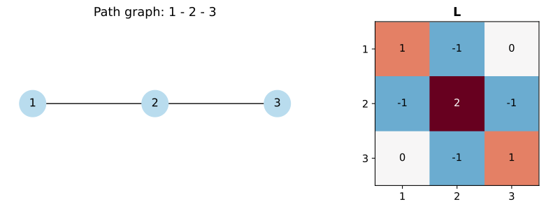
For the path $1-2-3$ with unit edge weights,
$$ \mathbf{A}=\begin{bmatrix}0&1&0\\1&0&1\\0&1&0\end{bmatrix},\quad \mathbf{D}=\begin{bmatrix}1&0&0\\0&2&0\\0&0&1\end{bmatrix},\quad \mathbf{L}=\begin{bmatrix}1&-1&0\\-1&2&-1\\0&-1&1\end{bmatrix}. $$
Expanding the determinant along the first row gives
$$ \begin{aligned} \det(\mathbf{L}-\lambda\mathbf{I}) &=(1-\lambda)\{(2-\lambda)(1-\lambda)-1\}-(1-\lambda)\\ &=(1-\lambda)\{(2-\lambda)(1-\lambda)-2\}\\ &=(1-\lambda)(\lambda^2-3\lambda)\\ &=-\lambda(\lambda-1)(\lambda-3). \end{aligned} $$
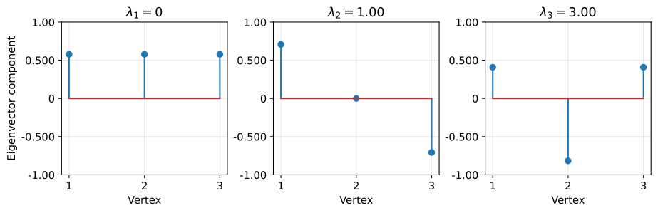
The eigenvalues are therefore $0,1,3$. The first row gives $u_2=(1-\lambda)u_1$, and the second gives $u_3=-u_1+(2-\lambda)u_2$. Setting $u_1=1$ and substituting each eigenvalue gives $(1,1,1)$, $(1,0,-1)$, and $(1,-2,1)$, all of which also satisfy the third row. Their lengths are $\sqrt3,\sqrt2,\sqrt6$, respectively, so
$$ \mathbf{u}_1=\frac1{\sqrt3}\begin{bmatrix}1\\1\\1\end{bmatrix},\quad \mathbf{u}_2=\frac1{\sqrt2}\begin{bmatrix}1\\0\\-1\end{bmatrix},\quad \mathbf{u}_3=\frac1{\sqrt6}\begin{bmatrix}1\\-2\\1\end{bmatrix}. $$
In the hand calculation, $u_i$ denotes the component at vertex $i$. In contrast, bold $\mathbf{u}_k$ denotes the entire eigenvector numbered $k$. The sign of the whole eigenvector can be reversed without changing its meaning.
path3 = nx.path_graph(range(1, 4))
L3 = laplacian(path3)
values3, vectors3, tol3 = spectrum(L3)

print("Laplacian:")
pprint(L3.astype(int))
print("Eigenvalues (display values within rounding error as zero):")
pprint(np.where(np.abs(values3) < tol3, 0, values3))

# Check the characteristic polynomial symbolically and display it as a formula.
lam = sp.Symbol("lambda")
symbolic_L = sp.Matrix(L3.astype(int))
polynomial = sp.factor((symbolic_L - lam * sp.eye(3)).det())
display(Latex(r"\(\det(\mathbf{L}-\lambda\mathbf{I})=" + sp.latex(polynomial) + r"\)"))
assert sp.expand(polynomial + lam * (lam - 1) * (lam - 3)) == 0
assert np.allclose(values3, [0, 1, 3])

# Independently check the eigenvalue equation and the squared differences across edges.
assert np.allclose(L3 @ vectors3, vectors3 * values3)
energies = np.array([
    sum((vectors3[i - 1, k] - vectors3[j - 1, k]) ** 2 for i, j in path3.edges)
    for k in range(3)
])
assert np.allclose(energies, values3)
print("Sum of squared differences across edges:")
pprint(np.where(np.abs(energies) < tol3, 0, energies))

fig, axes = plt.subplots(1, 2, figsize=(9, 3), layout="constrained")
nx.draw_networkx(path3, pos={i: (i, 0) for i in path3}, ax=axes[0],
                 node_color="#b9dcee", node_size=800)
axes[0].set_title("Path graph: 1 - 2 - 3")
axes[0].set_axis_off()
axes[1].imshow(L3, cmap="RdBu_r", vmin=-2, vmax=2)
for i in range(3):
    for j in range(3):
        axes[1].text(j, i, str(int(L3[i, j])), ha="center", va="center",
                     color="white" if L3[i, j] == 2 else "black")
axes[1].set(xticks=range(3), xticklabels=range(1, 4),
            yticks=range(3), yticklabels=range(1, 4), title=r"$\mathbf{L}$")
show_figure(fig, "01_path_and_laplacian")

fig, axes = plt.subplots(1, 3, figsize=(9.50, 3), layout="constrained")
for k, ax in enumerate(axes):
    vector = vectors3[:, k].copy()
    vector *= 1 if vector[0] >= 0 else -1  # Match the sign used in the hand calculation.
    ax.stem(range(1, 4), vector)
    value = 0 if abs(values3[k]) < tol3 else values3[k]
    ax.set(title=rf"$\lambda_{k + 1}={sig3(value)}$", xlabel="Vertex",
           xticks=range(1, 4), ylim=(-1, 1))
    ax.yaxis.set_major_formatter(tick_format)
    ax.grid(alpha=0.300)
axes[0].set_ylabel("Eigenvector component")
show_figure(fig, "02_eigenvectors")
Laplacian:
array([[ 1, -1,  0],
       [-1,  2, -1],
       [ 0, -1,  1]])
Eigenvalues (display values within rounding error as zero):
array([0, 1.00, 3.00])
$$ \det(\mathbf{L}-\lambda\mathbf{I})=- \lambda \left(\lambda - 3\right) \left(\lambda - 1\right) $$
Sum of squared differences across edges:
array([0, 1.00, 3.00])
4. Zero eigenvalues count connected components
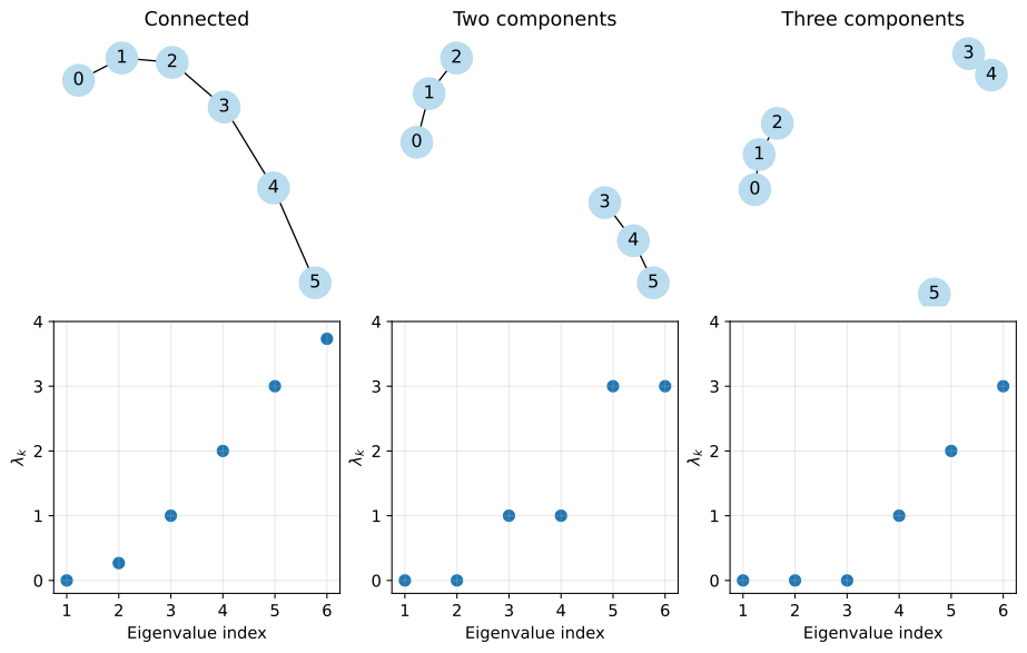
Each row sums to zero, so $\mathbf{L}\mathbf{1}=\mathbf{0}$. If $\mathbf{L}\mathbf{x}=\mathbf{0}$, the sum of squared differences from the previous section is zero, requiring $x_i=x_j$ across every edge with positive weight. Following these equalities along edges shows that the values are constant within each connected component.
Conversely, assigning a constant value to each component gives $\mathbf{L}\mathbf{x}=\mathbf{0}$. With $c$ components, we can choose $c$ independent constants, so the multiplicity of the zero eigenvalue is $c$. In ascending order, $0=\lambda_1\leq\lambda_2\leq\cdots\leq\lambda_n$, and the graph is connected if and only if $\lambda_2>0$.
Compare graphs with six vertices. Numerical zero tests require a tolerance, so an extremely small positive eigenvalue may be indistinguishable from zero.
cases = {
    "Connected": nx.path_graph(6),
    "Two components": nx.disjoint_union(nx.path_graph(3), nx.path_graph(3)),
    "Three components": nx.disjoint_union_all([
        nx.path_graph(3), nx.path_graph(2), nx.empty_graph(1)
    ]),
}
fig, axes = plt.subplots(2, 3, figsize=(9.50, 6), layout="constrained")
summary = []
for column, (name, graph) in enumerate(cases.items()):
    values, _, tolerance = spectrum(laplacian(graph))
    zeros = int(np.count_nonzero(np.abs(values) < tolerance))
    components = nx.number_connected_components(graph)
    assert zeros == components
    summary.append({"graph": name, "components": components, "zero_eigenvalues": zeros})

    nx.draw_networkx(graph, pos=nx.spring_layout(graph, seed=101),
                     ax=axes[0, column], node_color="#b9dcee", node_size=450)
    axes[0, column].set_title(name)
    axes[0, column].set_axis_off()
    shown = np.where(np.abs(values) < tolerance, 0, values)
    axes[1, column].scatter(range(1, 7), shown, s=55)
    axes[1, column].set(xlabel="Eigenvalue index", ylabel=r"$\lambda_k$",
                       xticks=range(1, 7), ylim=(-0.200, 4))
    axes[1, column].yaxis.set_major_locator(MaxNLocator(integer=True))
    axes[1, column].grid(alpha=0.300)
pprint(summary)
show_figure(fig, "03_components_and_spectra")
[{'components': 1, 'graph': 'Connected', 'zero_eigenvalues': 1},
 {'components': 2, 'graph': 'Two components', 'zero_eigenvalues': 2},
 {'components': 3, 'graph': 'Three components', 'zero_eigenvalues': 3}]
5. The second eigenvalue and weak connections
For a connected graph, $\mathbf{u}_1=\mathbf{1}/\sqrt n$. Expand a nonzero mean-zero vector $\mathbf{x}\ne\mathbf{0}$ as $\mathbf{x}=\sum_{k=2}^n c_k\mathbf{u}_k$. Orthonormality gives
$$ \frac{\mathbf{x}^{\mathsf T}\mathbf{L}\mathbf{x}}{\mathbf{x}^{\mathsf T}\mathbf{x}} =\frac{\sum_{k=2}^n\lambda_k c_k^2}{\sum_{k=2}^n c_k^2} \geq\frac{\lambda_2\sum_{k=2}^n c_k^2}{\sum_{k=2}^n c_k^2}=\lambda_2. $$
Equality holds for $\mathbf{x}=\mathbf{u}_2$, so
$$ \lambda_2=\min_{\mathbf{x}\ne\mathbf{0},\,\mathbf{x}^{\mathsf T}\mathbf{1}=0} \frac{\sum_{\{i,j\}\in E}w_{ij}(x_i-x_j)^2}{\sum_i x_i^2}. $$
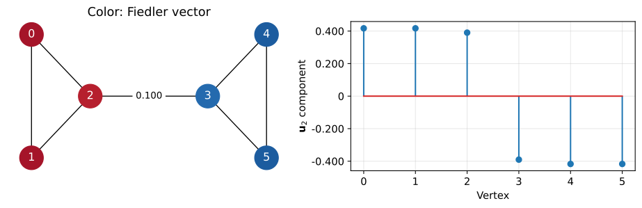
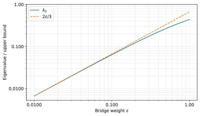
The value $\lambda_2$ is called algebraic connectivity. Join two triangles by one edge of weight $\varepsilon$, and assign 1 to vertices on one side and $-1$ to those on the other. Differences across internal edges are zero, the difference across the connecting edge is two, and the sum of squared vertex values is six. Therefore, $\lambda_2\leq\varepsilon(1-(-1))^2/6=2\varepsilon/3$.
A weak connection allows the two sides to have different values with little total variation across edges. In the plot, the sign of $\mathbf{u}_2$ also separates the two sides. However, multiplying every weight by $a>0$ multiplies both $\mathbf{L}$ and its eigenvalues by $a$. Comparisons between graphs therefore require consistent vertex counts and weight scales.
def joined_triangles(weight):
    graph = nx.disjoint_union(nx.complete_graph(3), nx.complete_graph(3))
    nx.set_edge_attributes(graph, 1, "weight")
    graph.add_edge(2, 3, weight=weight)
    return graph


bridge_weight = 0.100
bridge = joined_triangles(bridge_weight)
bridge_values, bridge_vectors, _ = spectrum(laplacian(bridge))
fiedler = bridge_vectors[:, 1]
fiedler *= 1 if fiedler[0] > 0 else -1
print("Connecting-edge weights and second eigenvalues:")
pprint({"weight": sig3(bridge_weight), "lambda_2": sig3(bridge_values[1])})

positions = {0: (0, 1), 1: (0, -1), 2: (1, 0),
             3: (3, 0), 4: (4, 1), 5: (4, -1)}
fig, axes = plt.subplots(1, 2, figsize=(9.50, 3), layout="constrained")
nx.draw_networkx(bridge, pos=positions, ax=axes[0], node_color=fiedler,
                 cmap=plt.cm.RdBu_r, vmin=-0.500, vmax=0.500, node_size=650, font_color="white")
nx.draw_networkx_edge_labels(bridge, positions, ax=axes[0],
                             edge_labels={(2, 3): sig3(bridge_weight)})
axes[0].set_title("Color: Fiedler vector")
axes[0].set_axis_off()
axes[1].stem(range(6), fiedler)
axes[1].set(xlabel="Vertex", ylabel=r"$\mathbf{u}_2$ component", xticks=range(6))
axes[1].yaxis.set_major_formatter(tick_format)
axes[1].grid(alpha=0.300)
show_figure(fig, "04_weak_bridge")

weights = np.geomspace(0.0100, 1, 60)
lambda2 = np.array([spectrum(laplacian(joined_triangles(w)))[0][1] for w in weights])
upper_bound = 2 * weights / 3
assert np.all(lambda2 <= upper_bound + 1e-12)
fig, ax = plt.subplots(figsize=(7, 4), layout="constrained")
ax.loglog(weights, lambda2, label=r"$\lambda_2$")
ax.loglog(weights, upper_bound, "--", label=r"$2\varepsilon/3$")
ax.set(xlabel=r"Bridge weight $\varepsilon$", ylabel="Eigenvalue / upper bound")
ax.set_xticks([0.0100, 0.100, 1])
ax.set_yticks([0.0100, 0.100, 1])
ax.xaxis.set_major_formatter(tick_format)
ax.yaxis.set_major_formatter(tick_format)
ax.xaxis.set_minor_formatter(plt.NullFormatter())
ax.yaxis.set_minor_formatter(plt.NullFormatter())
ax.legend()
ax.grid(which="both", alpha=0.300)
show_figure(fig, "05_bridge_weight_and_lambda2")
Connecting-edge weights and second eigenvalues:
{'lambda_2': '0.0638', 'weight': '0.100'}
6. Eigenvalues give diffusion decay rates
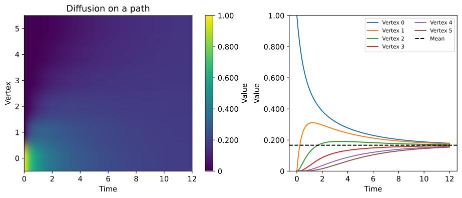
Consider diffusion in which each vertex value changes in proportion to its differences from neighboring values.
$$ \frac{dx_i}{dt}=\sum_j w_{ij}(x_j-x_i) =-(\mathbf{L}\mathbf{x})_i,\qquad \frac{d\mathbf{x}}{dt}=-\mathbf{L}\mathbf{x}. $$
Substitute $\mathbf{x}(t)=\sum_k c_k(t)\mathbf{u}_k$ and multiply both sides by $\mathbf{u}_k^{\mathsf T}$ to obtain $c_k^{\prime}(t)=-\lambda_k c_k(t)$. Using an integrating factor gives
$$ \frac{d}{dt}\{e^{\lambda_k t}c_k(t)\}=0 \quad\Rightarrow\quad c_k(t)=c_k(0)e^{-\lambda_k t}. $$
Therefore,
$$ \mathbf{x}(t)=\sum_{k=1}^n (\mathbf{u}_k^{\mathsf T}\mathbf{x}(0))e^{-\lambda_k t}\mathbf{u}_k. $$
For a connected graph, only the zero-eigenvalue component remains, and all values approach the initial mean $\bar{x}$. By orthonormality, the deviation from this mean satisfies
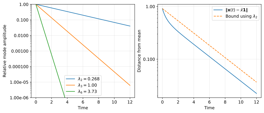
$$ \begin{aligned} \|\mathbf{x}(t)-\bar{x}\mathbf{1}\|^2 &=\sum_{k=2}^n c_k(0)^2e^{-2\lambda_k t}\\ &\leq e^{-2\lambda_2t}\sum_{k=2}^n c_k(0)^2\\ &=e^{-2\lambda_2t}\|\mathbf{x}(0)-\bar{x}\mathbf{1}\|^2. \end{aligned} $$
Taking square roots shows that the norm bound decays as $e^{-\lambda_2t}$. The slowest nonconstant component has time constant $1/\lambda_2$. Actual convergence is faster if that component is absent from the initial values. For a disconnected graph, values converge to the mean within each connected component.
graph6 = nx.path_graph(6)
L6 = laplacian(graph6)
values6, vectors6, tolerance6 = spectrum(L6)
times = np.linspace(0, 12, 241)
initial = np.array([1, 0, 0, 0, 0, 0], dtype=float)
coefficients = vectors6.T @ initial

# Decay each eigenvector component, then reconstruct the values at the vertices.
decay = np.exp(-values6[:, None] * times[None, :])
states = vectors6 @ (coefficients[:, None] * decay)
assert np.allclose(states[:, 0], initial)
assert np.allclose(states.sum(axis=0), initial.sum())
assert np.allclose(states[:, 60], expm(-L6 * times[60]) @ initial)
print("Second eigenvalue and time constant:")
pprint({"lambda_2": sig3(values6[1]), "1 / lambda_2": sig3(1 / values6[1])})

fig, axes = plt.subplots(1, 2, figsize=(9.50, 4), layout="constrained")
heatmap = axes[0].imshow(states, aspect="auto", origin="lower", cmap="viridis",
                         extent=[times[0], times[-1], -0.500, 5.50], vmin=0, vmax=1)
axes[0].set(xlabel="Time", ylabel="Vertex", yticks=range(6), title="Diffusion on a path")
fig.colorbar(heatmap, ax=axes[0], format=tick_format, label="Value")
for vertex in range(6):
    axes[1].plot(times, states[vertex], label=f"Vertex {vertex}")
axes[1].axhline(initial.mean(), color="black", linestyle="--", label="Mean")
axes[1].set(xlabel="Time", ylabel="Value", ylim=(0, 1))
axes[1].yaxis.set_major_formatter(tick_format)
axes[1].legend(ncol=2, fontsize=8)
show_figure(fig, "06_diffusion")

distance = np.linalg.norm(states - initial.mean(), axis=0)
bound = np.linalg.norm(initial - initial.mean()) * np.exp(-values6[1] * times)
assert np.all(distance <= bound + 1e-12)
fig, axes = plt.subplots(1, 2, figsize=(9.50, 4), layout="constrained")
for k in (1, 2, 5):
    axes[0].semilogy(times, decay[k], label=rf"$\lambda_{k + 1}={sig3(values6[k])}$")
axes[0].set(xlabel="Time", ylabel="Relative mode amplitude", ylim=(1e-6, 1))
axes[1].semilogy(times, distance, label=r"$\|\mathbf{x}(t)-\bar{x}\mathbf{1}\|$")
axes[1].semilogy(times, bound, "--", label=r"Bound using $\lambda_2$")
axes[1].set(xlabel="Time", ylabel="Distance from mean")
for ax in axes:
    ax.legend()
    ax.grid(alpha=0.300)
    ax.yaxis.set_major_formatter(tick_format)
    ax.yaxis.set_minor_formatter(plt.NullFormatter())
show_figure(fig, "07_decay_rates")
Second eigenvalue and time constant:
{'1 / lambda_2': '3.73', 'lambda_2': '0.268'}
Conclusion
We examined graph Laplacian eigenvalues through variation across edges, the number of connected components, and diffusion decay rates.
The number of zero eigenvalues equals the number of connected components. The second eigenvalue gives the minimum variation for normalized mean-zero vertex values and determines the slowest diffusion component in a connected graph. Normalized matrices require different treatment of eigenvalues and averages.