The Fiedler vector and spectral clustering (Rewritten from an earlier blog post)
Environment
Python 3.14.6, NumPy 2.5.4, SciPy 1.18.1, scikit-learn 1.9.1, NetworkX 3.7, Matplotlib 3.11.2 (Jupyter Notebook).
This article is a rewrite of a post from around 2013–2016, with calculations performed in the environment described above.
Overview
We use graph connections to divide data into groups. After deriving why the Fiedler vector appears, we move from a four-vertex example to spectral clustering. Finally, we partition two-moons data and compare the result with ordinary K-means.
Setup
Run the code in Jupyter Notebook from top to bottom. Round numbers to three significant digits only when displaying them.
import platform
from importlib.metadata import version
from pathlib import Path
from pprint import pprint

import matplotlib.pyplot as plt
import networkx as nx
import numpy as np
from IPython.display import Latex, display
from matplotlib.ticker import FuncFormatter
from matplotlib_inline.backend_inline import set_matplotlib_formats
from scipy.linalg import eigh
from scipy.sparse.csgraph import connected_components
from sklearn.cluster import KMeans, SpectralClustering
from sklearn.datasets import make_moons
from sklearn.metrics import adjusted_rand_score
from sklearn.neighbors import kneighbors_graph

%matplotlib inline
set_matplotlib_formats('svg')

print('Python:', platform.python_version())
for package in ('numpy', 'scipy', 'matplotlib', 'networkx', 'scikit-learn'):
    print(f'{package}: {version(package)}')

OUT = Path('102_nb_files')
OUT.mkdir(exist_ok=True)
COLORS = np.array(['#2369a1', '#cf5b32'])


def sig3(value):
    """Use three significant digits only for display, keeping trailing zeros."""
    return '0' if value == 0 else format(float(value), '#.3g')


np.set_printoptions(formatter={'float_kind': sig3})
plt.rcParams.update({'font.size': 11, 'svg.fonttype': 'none'})


def save_figure(fig, name):
    """Format tick labels and use the same figure for SVG saving and notebook display."""
    for ax in fig.axes:
        ax.xaxis.set_major_formatter(FuncFormatter(lambda value, _: sig3(value)))
        ax.yaxis.set_major_formatter(FuncFormatter(lambda value, _: sig3(value)))
    fig.savefig(OUT / name, format='svg', bbox_inches='tight')
    plt.show()
    plt.close(fig)
Python: 3.14.6
numpy: 2.5.4
scipy: 1.18.1
matplotlib: 3.11.2
networkx: 3.7
scikit-learn: 1.9.1
1. The graph Laplacian
Consider an undirected graph without self-loops. Its weight matrix $\mathbf{W}$ is symmetric, with $w_{ij}\geq0$. The degree $d_i$ is the sum of edge weights. Define the degree matrix $\mathbf{D}$ and Laplacian $\mathbf{L}$.
$$ d_i=\sum_jw_{ij},\quad \mathbf{D}=\operatorname{diag}(d_1,\ldots,d_n),\quad \mathbf{L}=\mathbf{D}-\mathbf{W} $$
For a real vector $\mathbf{x}$, symmetry gives the following rearrangement.
$$ \begin{aligned} \mathbf{x}^{\mathsf T}\mathbf{L}\mathbf{x} &=\sum_i d_i x_i^2-\sum_{i,j}w_{ij}x_ix_j\\ &=\frac12\sum_{i,j}w_{ij}x_i^2+\frac12\sum_{i,j}w_{ij}x_j^2-\sum_{i,j}w_{ij}x_ix_j\\ &=\frac12\sum_{i,j}w_{ij}(x_i-x_j)^2 =\sum_{i<j}w_{ij}(x_i-x_j)^2\geq0. \end{aligned} $$
Increasing the difference between vertices connected by a heavy edge increases this quantity more strongly. Each row sums to $d_i-\sum_jw_{ij}=0$, so $\mathbf{L}\mathbf{1}=\mathbf{0}$.
2. The Fiedler vector
Order the eigenvalues as $0=\lambda_1\leq\lambda_2\leq\cdots\leq\lambda_n$. For a connected graph, $\lambda_2>0$, and a corresponding unit eigenvector $\mathbf{v}_2$ is a Fiedler vector. Let $\mathbf{v}_j$ be orthonormal eigenvectors, with $\mathbf{v}_1=\mathbf{1}/\sqrt n$.
$$ \begin{aligned} \mathbf{x}&=\sum_{j=1}^n a_j\mathbf{v}_j,\\ \mathbf{x}^{\mathsf T}\mathbf{1}=0&\Rightarrow a_1=0,\qquad \mathbf{x}^{\mathsf T}\mathbf{x}=1\Rightarrow\sum_{j=2}^n a_j^2=1,\\ \mathbf{x}^{\mathsf T}\mathbf{L}\mathbf{x} &=\sum_{j=2}^n\lambda_j a_j^2 \geq\lambda_2\sum_{j=2}^n a_j^2=\lambda_2. \end{aligned} $$
Equality holds for $\mathbf{x}=\mathbf{v}_2$. Thus, among directions orthogonal to the constant vector, this direction minimizes variation across edges.
$$ \mathbf{v}_2\in\operatorname*{arg\,min}_{\mathbf{x}^{\mathsf T}\mathbf{1}=0,\;\mathbf{x}^{\mathsf T}\mathbf{x}=1}\mathbf{x}^{\mathsf T}\mathbf{L}\mathbf{x} $$
The connection to graph partitioning
Divide the vertex set into $A,B$, with $a=|A|$, $b=|B|$, and $n=a+b$. The total boundary weight is $c=\sum_{i\in A,j\in B}w_{ij}$. Set $f_i=\sqrt{b/a}$ for $i\in A$ and $f_i=-\sqrt{a/b}$ for $i\in B$. Then
$$ \begin{aligned} \mathbf{f}^{\mathsf T}\mathbf{1}&=a\sqrt{b/a}-b\sqrt{a/b}=0,\\ \mathbf{f}^{\mathsf T}\mathbf{f}&=a(b/a)+b(a/b)=n,\\ \mathbf{f}^{\mathsf T}\mathbf{L}\mathbf{f} &=c\left(\sqrt{b/a}+\sqrt{a/b}\right)^2 =c\frac{(a+b)^2}{ab},\\ \frac{\mathbf{f}^{\mathsf T}\mathbf{L}\mathbf{f}}{\mathbf{f}^{\mathsf T}\mathbf{f}} &=c\frac{a+b}{ab}=c\left(\frac1a+\frac1b\right) =\operatorname{RatioCut}(A,B). \end{aligned} $$
Removing the two-value restriction gives the eigenvalue minimization problem above. Splitting by sign is one way to turn the continuous solution back into a discrete partition, but it does not necessarily give the optimal RatioCut.
3. A four-vertex example
Give edges $(1,2)$ and $(3,4)$ weight one, and the middle edge $(2,3)$ weight $0.200$. The degree vector is $\mathbf{d}=(1,1.20,1.20,1)^{\mathsf T}$. Display the matrix and eigenpairs, and check the numerical errors.
def path_laplacian(weight):
    # Connect two strong edges with a weak middle edge.
    W = np.array([
        [0, 1, 0, 0],
        [1, 0, weight, 0],
        [0, weight, 0, 1],
        [0, 0, 1, 0],
    ], dtype=float)
    return W, np.diag(W.sum(axis=1)) - W


W, L = path_laplacian(0.200)
values, vectors = eigh(L)  # For symmetric matrices: ascending eigenvalues, eigenvectors in columns.
fiedler = vectors[:, 1].copy()
if fiedler[0] > 0:
    fiedler *= -1  # Align signs to make the figures easier to compare.
labels = (fiedler >= 0).astype(int)

rows = [' & '.join(sig3(x) for x in row) for row in L]
display(Latex(r'$$\mathbf{L}=\begin{bmatrix}'
              + r'\\'.join(rows) + r'\end{bmatrix}$$'))
pprint({'eigenvalues': values, 'Fiedler vector': fiedler, 'labels': labels})

residual = np.linalg.norm(L @ fiedler - values[1] * fiedler)
pprint({'eigenpair residual': sig3(residual),
        'orthogonality error': sig3(abs(fiedler.sum()))})
assert residual < 1e-12
assert abs(fiedler.sum()) < 1e-12
assert np.array_equal(labels, [0, 0, 1, 1])

# Compare the continuous minimum with the RatioCut obtained by splitting by sign.
A, B = labels == 0, labels == 1
cut = W[np.ix_(A, B)].sum()
ratio_cut = cut * (1 / A.sum() + 1 / B.sum())
display(Latex(r'$$\lambda_2\approx ' + sig3(values[1])
              + r'\leq\operatorname{RatioCut}(A,B)=' + sig3(ratio_cut) + r'$$'))
assert values[1] <= ratio_cut + 1e-12
$$\mathbf{L}=\begin{bmatrix}1.00 & -1.00 & 0 & 0\\-1.00 & 1.20 & -0.200 & 0\\0 & -0.200 & 1.20 & -1.00\\0 & 0 & -1.00 & 1.00\end{bmatrix}$$
{'Fiedler vector': array([-0.547, -0.448, 0.448, 0.547]),
 'labels': array([0, 0, 1, 1]),
 'eigenvalues': array([8.88e-16, 0.180, 2.00, 2.22])}
{'eigenpair residual': '4.10e-16', 'orthogonality error': '1.67e-15'}
$$\lambda_2\approx 0.180\leq\operatorname{RatioCut}(A,B)=0.200$$
graph = nx.from_numpy_array(W)
positions = {i: (i, 0) for i in range(4)}
fig, axes = plt.subplots(1, 2, figsize=(10, 3), layout='constrained')
nx.draw_networkx(
    graph, pos=positions, ax=axes[0], labels={i: i + 1 for i in range(4)},
    node_color=COLORS[labels], font_color='white', node_size=650,
    width=[3 * graph[u][v]['weight'] for u, v in graph.edges],
)
nx.draw_networkx_edge_labels(
    graph, pos=positions, ax=axes[0],
    edge_labels={(u, v): sig3(data['weight']) for u, v, data in graph.edges(data=True)},
)
axes[0].set_title('Graph and sign partition')
axes[0].set_axis_off()
heatmap = axes[1].imshow(W, cmap='Blues', vmin=0, vmax=1)
axes[1].set(xticks=range(4), yticks=range(4), xlabel='Vertex index (0-based)',
            ylabel='Vertex index (0-based)', title='Weight matrix')
fig.colorbar(heatmap, ax=axes[1])
save_figure(fig, '01_graph.svg')

fig, axes = plt.subplots(1, 2, figsize=(10, 3), layout='constrained')
axes[0].plot(range(1, 5), np.maximum(values, 0), 'o-')
axes[0].set(xlabel='Eigenvalue index', ylabel='Eigenvalue', xticks=range(1, 5))
axes[1].bar(range(1, 5), fiedler, color=COLORS[labels])
axes[1].axhline(0, color='black', linewidth=1)
axes[1].set(xlabel='Vertex', ylabel='Fiedler component', xticks=range(1, 5))
save_figure(fig, '02_eigenpairs.svg')
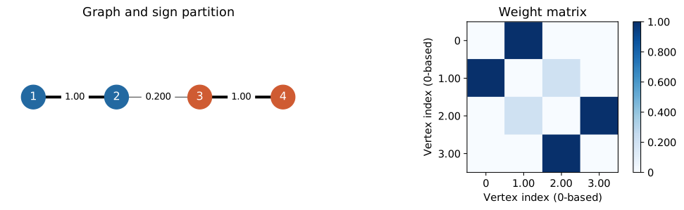
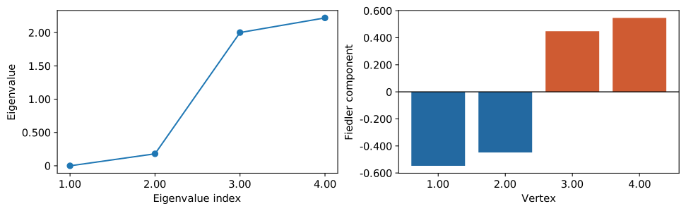
The Fiedler vector changes sign across the middle edge. Splitting by sign puts $\{1,2\}$ in one group and $\{3,4\}$ in the other, keeping each unit-weight edge within a group.
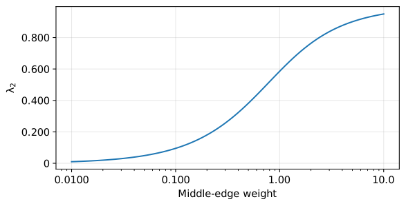
Now vary the middle-edge weight. The value $\lambda_2$ measures the strength of connectivity and approaches zero as the middle weight approaches zero. The overall sign of an eigenvector has no significance: reversing it leaves the partition unchanged.
bridge_weights = np.geomspace(0.0100, 10, 80)
second_values = np.array([
    eigh(path_laplacian(weight)[1], eigvals_only=True)[1]
    for weight in bridge_weights
])
fig, ax = plt.subplots(figsize=(6, 3), layout='constrained')
ax.semilogx(bridge_weights, second_values)
ax.set(xlabel='Middle-edge weight', ylabel=r'$\lambda_2$')
ax.grid(alpha=0.300)
save_figure(fig, '03_bridge_weight.svg')
4. Normalization and spectral clustering
To account for differences in degree, use $\operatorname{vol}(A)=\sum_{i\in A}d_i$ instead of the number of vertices. The corresponding objective is $\operatorname{Ncut}(A,B)=c/\operatorname{vol}(A)+c/\operatorname{vol}(B)$.
Assuming $d_i>0$, define the normalized Laplacian.
$$ \mathbf{L}_{\mathrm{sym}}=\mathbf{D}^{-1/2}\mathbf{L}\mathbf{D}^{-1/2}=\mathbf{I}-\mathbf{D}^{-1/2}\mathbf{W}\mathbf{D}^{-1/2} $$
Transforming an eigenvector $\mathbf{u}$ back to $\mathbf{f}=\mathbf{D}^{-1/2}\mathbf{u}$ gives
$$ \begin{aligned} \mathbf{D}^{-1/2}\mathbf{L}\mathbf{D}^{-1/2}\mathbf{u}&=\lambda\mathbf{u},\\ \mathbf{L}\mathbf{D}^{-1/2}\mathbf{u}&=\lambda\mathbf{D}^{1/2}\mathbf{u},\\ \mathbf{L}\mathbf{f}&=\lambda\mathbf{D}\mathbf{f}. \end{aligned} $$
This generalized eigenvalue problem corresponds to a continuous relaxation of Ncut. Form $\mathbf{F}=(\mathbf{f}_1,\ldots,\mathbf{f}_k)$ from the $k$ eigenvectors with smallest eigenvalues, including the zero-eigenvalue column, and pass its rows to K-means. This is one normalized approach and should be distinguished from the unnormalized $\mathbf{v}_2$.
5. Partitioning two-moons data
Generate 240 points and connect each point to its eight nearest neighbors. Add an edge if either point considers the other a neighbor, symmetrizing with $\mathbf{W}=\max(\mathbf{C},\mathbf{C}^{\mathsf T})$. Use the true labels only for comparison. The adjusted Rand index (ARI) is unchanged by relabeling and equals one for a perfect match.
X, truth = make_moons(n_samples=240, noise=0.0600, random_state=102)
C = kneighbors_graph(X, n_neighbors=8, mode='connectivity', include_self=False)
affinity = C.maximum(C.T)
components = connected_components(affinity, directed=False, return_labels=False)
print('Number of connected components:', components)
assert components == 1

# This is a small example, so form the normalized Laplacian explicitly as a dense matrix.
W_moon = affinity.toarray()
degree = W_moon.sum(axis=1)
assert np.all(degree > 0)
inv_sqrt = 1 / np.sqrt(degree)
L_sym = np.eye(len(X)) - inv_sqrt[:, None] * W_moon * inv_sqrt[None, :]
moon_values, U = eigh(L_sym)
embedding = inv_sqrt[:, None] * U[:, :2]
manual = KMeans(n_clusters=2, n_init=20, random_state=102).fit_predict(embedding)

# Pass the same similarity matrix to scikit-learn; this is not a distance matrix.
spectral = SpectralClustering(
    n_clusters=2, affinity='precomputed', eigen_solver='arpack',
    assign_labels='kmeans', n_init=20, random_state=102,
).fit_predict(affinity)
ordinary = KMeans(n_clusters=2, n_init=20, random_state=102).fit_predict(X)
pprint({
    'ordinary K-means ARI': sig3(adjusted_rand_score(truth, ordinary)),
    'explicit eigensolver ARI': sig3(adjusted_rand_score(truth, manual)),
    'SpectralClustering ARI': sig3(adjusted_rand_score(truth, spectral)),
    'ARI between implementations': sig3(adjusted_rand_score(manual, spectral)),
})
assert adjusted_rand_score(manual, spectral) > 0.990

fig, axes = plt.subplots(1, 3, figsize=(12, 3), layout='constrained')
for ax, group, title in zip(
    axes, (truth, ordinary, spectral), ('Reference labels', 'K-means', 'Spectral clustering')
):
    ax.scatter(X[:, 0], X[:, 1], c=COLORS[group], s=16)
    ax.set(title=title, xlabel=r'$x_1$', ylabel=r'$x_2$', aspect='equal')
save_figure(fig, '04_moons.svg')

# Examine the second generalized eigenvector and the ordered normalized eigenvalues.
fig, axes = plt.subplots(1, 2, figsize=(10, 3), layout='constrained')
order = np.argsort(embedding[:, 1])
axes[0].scatter(np.arange(len(X)), embedding[order, 1],
                c=COLORS[truth[order]], s=14)
axes[0].set(xlabel='Rank by second component', ylabel='Second component')
axes[1].plot(range(1, 11), np.maximum(moon_values[:10], 0), 'o-')
axes[1].set(xlabel='Eigenvalue index', ylabel='Normalized eigenvalue', xticks=[1, 2, 4, 6, 8, 10])
save_figure(fig, '05_embedding.svg')
Number of connected components: 1
{'SpectralClustering ARI': '0.983',
 'ARI between implementations': '1.00',
 'explicit eigensolver ARI': '0.983',
 'ordinary K-means ARI': '0.222'}
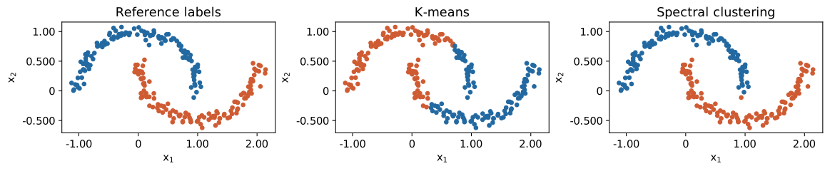
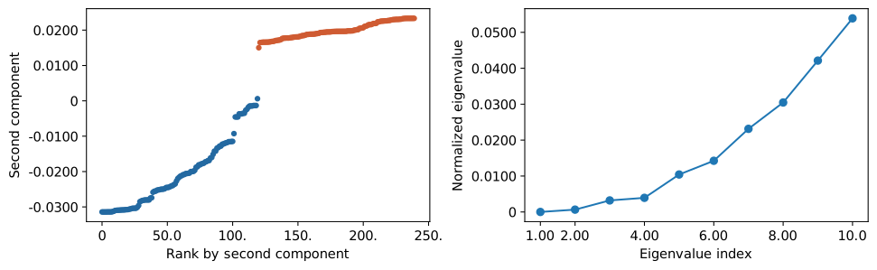
With these settings, spectral clustering follows the moon shapes more closely than ordinary K-means. Results depend on the number of neighbors and the noise level. Too few neighbors can disconnect the graph, while too many can create more edges between different groups.
A disconnected graph has multiple zero eigenvalues, so using only the second eigenvector to choose a partition is unstable. Eigenvectors are also nonunique when eigenvalues are repeated. For large data sets, avoid dense matrices and use a sparse eigensolver.
Conclusion
We explained the Fiedler vector through a continuous relaxation of RatioCut and implemented spectral clustering using a normalized Laplacian.
Eigenvectors provide numerical representations of graph vertices. When assessing a partition, examine the definition of similarity and the number of connected components as well as the eigenvalues.