Graph diffusion and Personalized PageRank (Rewritten from an earlier blog post)
Environment
Python 3.14.6, NumPy 2.5.4, SciPy 1.18.1, SymPy 1.14.0, NetworkX 3.7, Matplotlib 3.11.2 (Jupyter Notebook).
This article is a rewrite of a post from around 2013–2016, with calculations performed in the environment described above.
Overview
Graph diffusion combines the results of walks of different lengths using weights. Personalized PageRank (PPR) uses geometric weights. We derive its formulas from a transition matrix, work through a three-vertex example, implement it with sparse matrices, and compare restart probabilities and starting points. Finally, we examine how it differs from a heat kernel.
Setup
Run the code in Jupyter Notebook from top to bottom. Round numbers to three significant digits only when displaying them.
import platform
from importlib.metadata import version
from pathlib import Path
from pprint import pprint

import matplotlib.pyplot as plt
import networkx as nx
import numpy as np
import sympy as sp
from IPython.display import Latex, SVG, display
from matplotlib.colors import Normalize
from matplotlib.ticker import FuncFormatter, MaxNLocator
from scipy.linalg import expm
from scipy.sparse import csc_array, diags_array, eye_array
from scipy.sparse.linalg import spsolve
from scipy.stats import poisson

print("Python:", platform.python_version())
for package in ("numpy", "scipy", "matplotlib", "networkx", "sympy"):
    print(f"{package}: {version(package)}")

OUT = Path("105_nb_files")
OUT.mkdir(exist_ok=True)
plt.rcParams.update({"font.size": 11, "svg.fonttype": "path"})


def sig3(value):
    """Display nonzero numbers with three significant digits, including trailing zeros."""
    return "0" if value == 0 else f"{float(value):#.3g}"


np.set_printoptions(formatter={"float_kind": sig3})
tick_format = FuncFormatter(lambda value, _: sig3(value))


def show_math(source):
    # Convert key formulas from \(...\) to $$...$$ for use in HTML output too.
    display(Latex(source.replace(r"\(", "$$").replace(r"\)", "$$")))


def save_svg(fig, name):
    """Save an SVG and embed the same figure in the notebook output."""
    target = OUT / name
    fig.savefig(target, format="svg", bbox_inches="tight")
    plt.close(fig)
    display(SVG(filename=str(target)))
Python: 3.14.6
numpy: 2.5.4
scipy: 1.18.1
matplotlib: 3.11.2
networkx: 3.7
sympy: 1.14.0
1. From random walks to diffusion
Consider an undirected graph with nonnegative weights and no isolated vertices. Let $\mathbf{A}$ be its adjacency matrix, $d_j=\sum_i A_{ij}$ its degrees, and $\mathbf{D}=\operatorname{diag}(d_0,\ldots,d_{n-1})$ its degree matrix. Represent probabilities as column vectors.
$$ \mathbf{P}=\mathbf{A}\mathbf{D}^{-1},\qquad P_{ij}=\frac{A_{ij}}{d_j},\qquad \sum_iP_{ij}=1. $$
The entry $P_{ij}$ is the probability of moving from vertex $j$ to vertex $i$. For a starting distribution $\mathbf{s}\geq\mathbf{0}$ with $\mathbf{1}^{\mathsf T}\mathbf{s}=1$, the distribution after one step is $\mathbf{P}\mathbf{s}$ and after two steps is $\mathbf{P}^2\mathbf{s}$.
$$ \mathbf{S}=\sum_{k=0}^{\infty}\theta_k\mathbf{P}^k,\qquad \mathbf{x}=\mathbf{S}\mathbf{s},\qquad \theta_k\geq0,\quad\sum_{k=0}^{\infty}\theta_k=1. $$
This is the arrival distribution when the number of steps $k$ is chosen with probability $\theta_k$.
2. Deriving PPR
At each step, restart at a vertex drawn from the starting distribution $\mathbf{s}$ with probability $\alpha\in(0,1)$, or move along an edge with probability $\beta=1-\alpha$. Setting $\mathbf{p}^{(0)}=\mathbf{s}$ gives
$$ \begin{aligned} \mathbf{p}^{(t+1)}&=\alpha\mathbf{s}+\beta\mathbf{P}\mathbf{p}^{(t)},\\ \mathbf{p}^{(1)}&=\alpha\mathbf{s}+\beta\mathbf{P}\mathbf{s},\\ \mathbf{p}^{(2)}&=\alpha\mathbf{s}+\alpha\beta\mathbf{P}\mathbf{s}+\beta^2\mathbf{P}^2\mathbf{s},\\ \mathbf{p}^{(t)}&=\alpha\sum_{k=0}^{t-1}\beta^k\mathbf{P}^k\mathbf{s} +\beta^t\mathbf{P}^t\mathbf{s}. \end{aligned} $$
The entries of the last term sum to $\beta^t$, which tends to zero. For the limit $\mathbf{p}$,
$$ \begin{aligned} \mathbf{p}&=\alpha\mathbf{s}+\beta\mathbf{P}\mathbf{p},\\ (\mathbf{I}-\beta\mathbf{P})\mathbf{p}&=\alpha\mathbf{s},\\ \mathbf{p}&=\alpha(\mathbf{I}-\beta\mathbf{P})^{-1}\mathbf{s} =\sum_{k=0}^{\infty}\alpha\beta^k\mathbf{P}^k\mathbf{s}. \end{aligned} $$
Since $\|\beta\mathbf{P}\|_1=\beta<1$, the inverse exists and the solution is unique. The weights are $\theta_k=\alpha\beta^k$ and sum to $\alpha/(1-\beta)=1$. Therefore, $\mathbf{p}$ is also a nonnegative probability distribution whose entries sum to one.
3. A three-vertex calculation
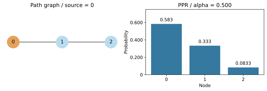
Use the path $0-1-2$ and set $\mathbf{s}=(1,0,0)^{\mathsf T}$. The transition matrix and component equations are as follows.
# Keep exact fractions and compare the hand calculation with the linear-system solution.
P3 = sp.Matrix([[0, sp.Rational(1, 2), 0],
                [1, 0, 1],
                [0, sp.Rational(1, 2), 0]])
s3 = sp.Matrix([1, 0, 0])
show_math(r"\(\mathbf{P}=" + sp.latex(P3) + r"\)")
show_math(r"\(\begin{aligned}"
          r"p_0&=\alpha+\beta p_1/2,&"
          r"p_1&=\beta(p_0+p_2),&p_2&=\beta p_1/2.\\"
          r"p_0+p_2&=\alpha+\beta p_1,\\"
          r"p_1&=\alpha\beta+\beta^2p_1,\\"
          r"p_1&=\frac{\alpha\beta}{1-\beta^2}"
          r"=\frac{(1-\beta)\beta}{(1-\beta)(1+\beta)}"
          r"=\frac{\beta}{1+\beta},\\"
          r"p_2&=\frac{\beta^2}{2(1+\beta)},\qquad "
          r"p_0=\alpha+\frac{\beta^2}{2(1+\beta)}."
          r"\end{aligned}\)")

alpha3 = sp.Rational(1, 2)
beta3 = 1 - alpha3
exact3 = (sp.eye(3) - beta3 * P3).inv() * (alpha3 * s3)
assert exact3 == sp.Matrix([sp.Rational(7, 12), sp.Rational(1, 3),
                           sp.Rational(1, 12)])
show_math(r"\(\alpha=\frac12,\quad p_1=\frac{1/2}{1+1/2}=\frac13,"
          r"\quad p_2=\frac12\frac{1/3}{2}=\frac1{12},"
          r"\quad p_0=\frac12+\frac1{12}=\frac7{12}.\)")
show_math(r"\(\mathbf{p}=" + sp.latex(exact3) + r"\)")
p3 = np.array(exact3, dtype=float).ravel()
pprint(p3)

fig, axes = plt.subplots(1, 2, figsize=(9, 3), layout="constrained")
nx.draw_networkx(nx.path_graph(3), pos={i: (i, 0) for i in range(3)},
                 ax=axes[0], node_color=["#e6a15a", "#b9dcee", "#b9dcee"],
                 node_size=900)
axes[0].set_title("Path graph / source = 0")
axes[0].set_axis_off()
axes[1].bar(range(3), p3, color="#3679a0")
axes[1].bar_label(axes[1].containers[0], labels=[sig3(x) for x in p3], padding=4)
axes[1].set(xlabel="Node", ylabel="Probability", title="PPR / alpha = 0.500",
            ylim=(0, 0.750), xticks=range(3))
axes[1].yaxis.set_major_formatter(tick_format)
save_svg(fig, "01_three_node_solution.svg")
$$\mathbf{P}=\left[\begin{matrix}0 & \frac{1}{2} & 0\\1 & 0 & 1\\0 & \frac{1}{2} & 0\end{matrix}\right]$$
$$\begin{aligned}p_0&=\alpha+\beta p_1/2,&p_1&=\beta(p_0+p_2),&p_2&=\beta p_1/2.\\p_0+p_2&=\alpha+\beta p_1,\\p_1&=\alpha\beta+\beta^2p_1,\\p_1&=\frac{\alpha\beta}{1-\beta^2}=\frac{(1-\beta)\beta}{(1-\beta)(1+\beta)}=\frac{\beta}{1+\beta},\\p_2&=\frac{\beta^2}{2(1+\beta)},\qquad p_0=\alpha+\frac{\beta^2}{2(1+\beta)}.\end{aligned}$$
$$\alpha=\frac12,\quad p_1=\frac{1/2}{1+1/2}=\frac13,\quad p_2=\frac12\frac{1/3}{2}=\frac1{12},\quad p_0=\frac12+\frac1{12}=\frac7{12}.$$
$$\mathbf{p}=\left[\begin{matrix}\frac{7}{12}\\\frac{1}{3}\\\frac{1}{12}\end{matrix}\right]$$
array([0.583, 0.333, 0.0833])
4. Restart probability and spread
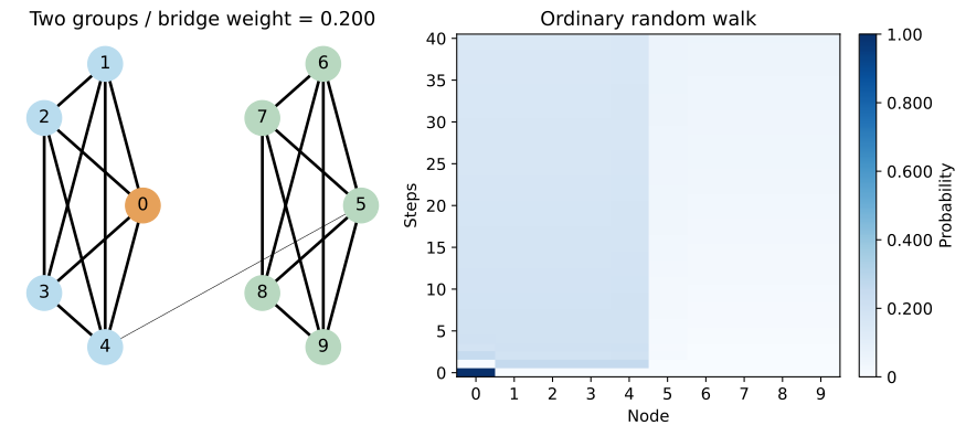
Build two complete graphs with five vertices each, joined by an edge between vertices 4 and 5 of weight $0.200$. All other edges have weight one. Start at vertex 0. An ordinary walk gradually spreads to the right-hand group.
Differentiating the geometric series gives the mean number of steps $K$ mixed by PPR.
$$ \begin{aligned} \sum_{k=0}^{\infty}\beta^k&=(1-\beta)^{-1},\\ \sum_{k=1}^{\infty}k\beta^{k-1}&=(1-\beta)^{-2},\\ \mathbb{E}[K]&=\alpha\beta\sum_{k=1}^{\infty}k\beta^{k-1} =\frac{\alpha\beta}{(1-\beta)^2}=\frac{1-\alpha}{\alpha}. \end{aligned} $$
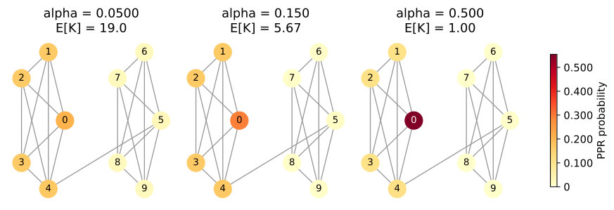
Larger $\alpha$ gives more weight to shorter walks. For example, $\alpha=0.0500$ gives a mean of 19 steps, while $\alpha=0.500$ gives a mean of one step.
G = nx.disjoint_union(nx.complete_graph(5), nx.complete_graph(5))
nx.set_edge_attributes(G, 1, "weight")
G.add_edge(4, 5, weight=0.200)
nodes = list(range(10))
A = nx.to_scipy_sparse_array(G, nodelist=nodes, weight="weight", format="csc")
degrees = np.asarray(A.sum(axis=0)).ravel()
assert np.all(degrees > 0)  # This example contains no isolated vertices.
P = csc_array(A @ diags_array(1 / degrees))
n = len(nodes)
s = np.zeros(n)
s[0] = 1
assert np.allclose(np.asarray(P.sum(axis=0)).ravel(), 1)

# Place the two groups apart and keep these positions in all later plots.
angle = np.linspace(0, 2 * np.pi, 5, endpoint=False)
pos = {i: (np.cos(angle[i]), np.sin(angle[i])) for i in range(5)}
pos.update({i + 5: (4 + np.cos(angle[i]), np.sin(angle[i])) for i in range(5)})

walk = [s.copy()]
for _ in range(40):
    walk.append(P @ walk[-1])
walk = np.asarray(walk)
assert np.allclose(walk.sum(axis=1), 1)

fig, axes = plt.subplots(1, 2, figsize=(9, 4), layout="constrained")
nx.draw_networkx(G, pos=pos, ax=axes[0], node_size=550,
                 node_color=["#e6a15a"] + ["#b9dcee"] * 4 + ["#b8d8c0"] * 5,
                 width=[2 * G[u][v]["weight"] for u, v in G.edges])
axes[0].set_title("Two groups / bridge weight = 0.200")
axes[0].set_axis_off()
im = axes[1].imshow(walk, aspect="auto", origin="lower", cmap="Blues",
                    extent=(-0.500, 9.50, -0.500, 40.5), vmin=0, vmax=1)
axes[1].set(xlabel="Node", ylabel="Steps", title="Ordinary random walk",
            xticks=nodes)
axes[1].yaxis.set_major_locator(MaxNLocator(integer=True))
fig.colorbar(im, ax=axes[1], label="Probability", format=tick_format)
save_svg(fig, "02_graph_and_random_walk.svg")
Do not form the inverse in the implementation. Instead, solve $(\mathbf{I}-\beta\mathbf{P})\mathbf{p}=\alpha\mathbf{s}$ with scipy.sparse.linalg.spsolve. Use the same color range in all three plots.
def ppr_solve(transition, source, alpha):
    """Compute PPR from a column-stochastic matrix by solving a sparse linear system."""
    if not 0 < alpha < 1:
        raise ValueError("alpha must be between 0 and 1")
    coefficient = eye_array(transition.shape[0], format="csc") - (1 - alpha) * transition
    return spsolve(coefficient, alpha * source)


alphas = (0.0500, 0.150, 0.500)
profiles = {alpha: ppr_solve(P, s, alpha) for alpha in alphas}
for alpha, probability in profiles.items():
    assert np.all(probability >= 0)
    assert np.isclose(probability.sum(), 1)
    assert np.linalg.norm(probability - alpha * s - (1 - alpha) * (P @ probability), 1) < 1.00e-12
    pprint({"alpha": sig3(alpha), "mean steps": sig3((1 - alpha) / alpha),
            "right-group probability": sig3(probability[5:].sum())})

fig, axes = plt.subplots(1, 3, figsize=(9, 3), layout="constrained")
vmax = max(float(p.max()) for p in profiles.values())
for ax, alpha in zip(axes, alphas):
    probability = profiles[alpha]
    nx.draw_networkx(G, pos=pos, ax=ax, node_size=350, node_color=probability,
                     cmap=plt.cm.YlOrRd, vmin=0, vmax=vmax,
                     edge_color="#999999", with_labels=False)
    # Use white labels on dark vertices to keep their numbers readable.
    for node in nodes:
        nx.draw_networkx_labels(G, pos, labels={node: str(node)}, ax=ax,
                                font_size=10,
                                font_color="white" if probability[node] / vmax > 0.550 else "black")
    ax.set_title(f"alpha = {sig3(alpha)}\nE[K] = {sig3((1 - alpha) / alpha)}")
    ax.set_axis_off()
fig.colorbar(plt.cm.ScalarMappable(norm=Normalize(0, vmax), cmap="YlOrRd"),
             ax=list(axes), label="PPR probability", format=tick_format, shrink=0.800)
save_svg(fig, "03_restart_probability.svg")
{'alpha': '0.0500', 'right-group probability': '0.125', 'mean steps': '19.0'}
{'alpha': '0.150', 'right-group probability': '0.0419', 'mean steps': '5.67'}
{'alpha': '0.500', 'right-group probability': '0.00513', 'mean steps': '1.00'}
5. Iteration and convergence
For the error $\mathbf{e}^{(t)}=\mathbf{p}^{(t)}-\mathbf{p}$, the restart terms cancel. Here, $\|\mathbf{v}\|_1=\sum_i|v_i|$.
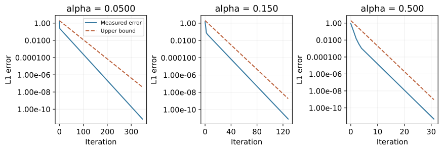
$$ \begin{aligned} \mathbf{e}^{(t+1)}&=\beta\mathbf{P}\mathbf{e}^{(t)},\\ \|\mathbf{e}^{(t)}\|_1&\leq\beta^t\|\mathbf{s}-\mathbf{p}\|_1\leq2\beta^t. \end{aligned} $$
PPR iteration converges regardless of connectivity or whether the ordinary walk converges. Use the residual $\mathbf{r}=\mathbf{q}-\alpha\mathbf{s}-\beta\mathbf{P}\mathbf{q}$ as the stopping criterion. Since $(\mathbf{I}-\beta\mathbf{P})(\mathbf{q}-\mathbf{p})=\mathbf{r}$, the error satisfies $\|\mathbf{q}-\mathbf{p}\|_1\leq\sum_{k\geq0}\beta^k\|\mathbf{r}\|_1=\|\mathbf{r}\|_1/\alpha$.
The alpha argument in NetworkX is the probability of continuing the walk, so pass 1 - alpha here. Compare the direct solution, iterative solution, and NetworkX result.
def ppr_iterate(transition, source, alpha, tol=1.00e-11, max_iter=5000):
    probability = source.copy()
    history = [probability.copy()]
    for _ in range(max_iter):
        probability = alpha * source + (1 - alpha) * (transition @ probability)
        history.append(probability.copy())
        residual = probability - alpha * source - (1 - alpha) * (transition @ probability)
        if np.linalg.norm(residual, 1) / alpha <= tol:
            return probability, np.asarray(history)
    raise RuntimeError("Did not converge within the iteration limit")


fig, axes = plt.subplots(1, 3, figsize=(9, 3), layout="constrained")
for ax, alpha in zip(axes, alphas):
    direct = profiles[alpha]
    iterative, history = ppr_iterate(P, s, alpha)
    reference = nx.pagerank(G, alpha=1 - alpha,
                            personalization={i: float(s[i]) for i in nodes},
                            tol=1.00e-14, max_iter=5000, weight="weight")
    reference_array = np.array([reference[i] for i in nodes])
    error = np.linalg.norm(history - direct, ord=1, axis=1)
    steps = np.arange(len(history))
    bound = 2 * (1 - alpha) ** steps
    np.testing.assert_allclose(iterative, direct, atol=1.00e-11, rtol=0)
    np.testing.assert_allclose(reference_array, direct, atol=1.00e-11, rtol=0)
    assert np.all(error <= bound + 1.00e-14)
    pprint({"alpha": sig3(alpha), "iterations": len(history) - 1,
            "L1 error": sig3(error[-1]),
            "difference from NetworkX": sig3(np.linalg.norm(reference_array - direct, 1))})
    ax.semilogy(steps, error, color="#3679a0", label="Measured error")
    ax.semilogy(steps, bound, "--", color="#bb613c", label="Upper bound")
    ax.set(xlabel="Iteration", ylabel="L1 error", title=f"alpha = {sig3(alpha)}")
    ax.xaxis.set_major_locator(MaxNLocator(nbins=4, integer=True))
    ax.yaxis.set_major_formatter(tick_format)
    ax.grid(alpha=0.200)
axes[0].legend(fontsize=8)
save_svg(fig, "04_iteration_convergence.svg")
{'L1 error': '7.27e-12', 'difference from NetworkX': '1.34e-12', 'alpha': '0.0500', 'iterations': 347}
{'L1 error': '8.07e-12', 'difference from NetworkX': '4.78e-13', 'alpha': '0.150', 'iterations': 128}
{'L1 error': '4.82e-12', 'difference from NetworkX': '5.06e-14', 'alpha': '0.500', 'iterations': 31}
Each sparse matrix-vector update costs $O(|E|+n)$. We store the history for plotting, but only the latest vector is needed for large graphs.
6. Changing the starting distribution
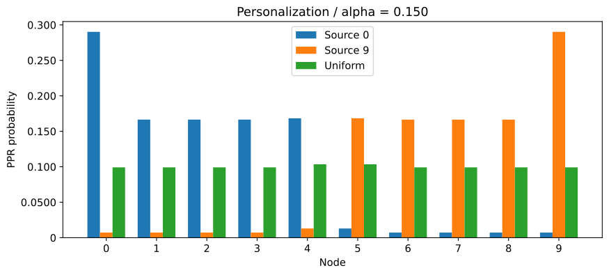
Change $\mathbf{s}$ to a point mass at vertex 0, a point mass at vertex 9, or a uniform distribution. Even on the same graph, PPR rankings depend on the starting distribution. In recommendations, normalized browsing histories could define $\mathbf{s}$, but the resulting values are arrival probabilities on the graph, not purchase probabilities.
alpha = 0.150
s_right = np.zeros(n)
s_right[9] = 1
sources = {"Source 0": s, "Source 9": s_right, "Uniform": np.ones(n) / n}
fig, ax = plt.subplots(figsize=(9, 4), layout="constrained")
width = 0.250
for offset, (label, source) in enumerate(sources.items()):
    probability = ppr_solve(P, source, alpha)
    assert np.isclose(probability.sum(), 1)
    ax.bar(np.arange(n) + (offset - 1) * width, probability, width=width, label=label)
    # Array entries follow vertices 0 through 9. Do not assign fine rankings to tied vertices.
    print(f"{label} (vertices 0 through 9)")
    pprint(probability)
ax.set(xlabel="Node", ylabel="PPR probability", xticks=nodes,
       title="Personalization / alpha = 0.150")
ax.yaxis.set_major_formatter(tick_format)
ax.legend()
save_svg(fig, "05_personalization.svg")
Source 0 (vertices 0 through 9)
array([0.290, 0.167, 0.167, 0.167, 0.168, 0.0130, 0.00724, 0.00724,
       0.00724, 0.00724])
Source 9 (vertices 0 through 9)
array([0.00724, 0.00724, 0.00724, 0.00724, 0.0130, 0.168, 0.167, 0.167,
       0.167, 0.290])
Uniform (vertices 0 through 9)
array([0.0991, 0.0991, 0.0991, 0.0991, 0.103, 0.103, 0.0991, 0.0991,
       0.0991, 0.0991])
7. Comparing with a heat kernel
Here, use $\mathbf{L}=\mathbf{I}-\mathbf{P}$. This is a degree-normalized probability diffusion operator and differs from $\mathbf{D}-\mathbf{A}$. The continuous-time equation gives
$$ \begin{aligned} \frac{d\mathbf{x}(\tau)}{d\tau}&=-\mathbf{L}\mathbf{x}(\tau),\quad\mathbf{x}(0)=\mathbf{s},\\ \mathbf{x}(\tau)&=e^{-\tau(\mathbf{I}-\mathbf{P})}\mathbf{s} =e^{-\tau}e^{\tau\mathbf{P}}\mathbf{s}\\ &=\sum_{k=0}^{\infty}e^{-\tau}\frac{\tau^k}{k!}\mathbf{P}^k\mathbf{s}. \end{aligned} $$
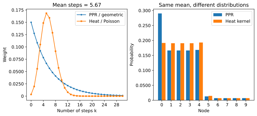
The step counts have a Poisson distribution with mean $\tau$. Even when $\tau=(1-\alpha)/\alpha$, its weights differ from geometric weights, so the arrival distributions differ. Compare these two diffusion methods described by Gasteiger et al. (2019) on the same graph.
alpha = 0.150
tau = (1 - alpha) / alpha
ppr = profiles[alpha]
# With only ten vertices, compute the matrix exponential directly. Use expm_multiply for large graphs.
heat = expm(-tau * (np.eye(n) - P.toarray())) @ s
assert np.all(heat >= -1.00e-14)
assert np.isclose(heat.sum(), 1)

# Independently approximate the infinite sums to check the matrix exponential and direct PPR solution.
k_check = np.arange(501)
weights_ppr = alpha * (1 - alpha) ** k_check
weights_heat = poisson.pmf(k_check, mu=tau)
power = s.copy()
series_ppr, series_heat = np.zeros(n), np.zeros(n)
for w_ppr, w_heat in zip(weights_ppr, weights_heat):
    series_ppr += w_ppr * power
    series_heat += w_heat * power
    power = P @ power
np.testing.assert_allclose(series_ppr, ppr, atol=1.00e-12, rtol=0)
np.testing.assert_allclose(series_heat, heat, atol=1.00e-12, rtol=0)
assert np.isclose(k_check @ weights_ppr, tau)
assert np.isclose(k_check @ weights_heat, tau)
pprint({"mean steps": sig3(tau), "PPR probability at source": sig3(ppr[0]),
        "heat probability at source": sig3(heat[0]),
        "L1 distance between distributions": sig3(np.linalg.norm(ppr - heat, 1))})

fig, axes = plt.subplots(1, 2, figsize=(9, 4), layout="constrained")
# The left plot shows up to 30 steps; this cutoff is not used in the right-hand calculation.
k = np.arange(31)
axes[0].plot(k, weights_ppr[:31], "o-", label="PPR / geometric", markersize=3)
axes[0].plot(k, weights_heat[:31], "s-", label="Heat / Poisson", markersize=3)
axes[0].set(xlabel="Number of steps k", ylabel="Weight", title=f"Mean steps = {sig3(tau)}")
axes[0].xaxis.set_major_locator(MaxNLocator(integer=True))
axes[1].bar(np.arange(n) - 0.200, ppr, width=0.400, label="PPR")
axes[1].bar(np.arange(n) + 0.200, heat, width=0.400, label="Heat kernel")
axes[1].set(xlabel="Node", ylabel="Probability", xticks=nodes,
            title="Same mean, different distributions")
for ax in axes:
    ax.yaxis.set_major_formatter(tick_format)
    ax.legend()
save_svg(fig, "06_ppr_and_heat_kernel.svg")
print("Checked the hand calculation, three PPR methods, and series expansions.")
{'heat probability at source': '0.192',
 'PPR probability at source': '0.290',
 'L1 distance between distributions': '0.198',
 'mean steps': '5.67'}
Checked the hand calculation, three PPR methods, and series expansions.
Conclusion
We defined graph diffusion as a mixture of distributions after different numbers of steps, then derived PPR and examined how to compute it.
PPR uses the restart probability to control step-count weights and the starting distribution to specify vertices of interest. A heat kernel mixes step counts with Poisson weights, so the results differ even at the same mean number of steps. Implementations must use a consistent transition-matrix orientation and definition of alpha.