Heat kernels and diffusion on graphs (Rewritten from an earlier blog post)
Environment
Python 3.14.6, NumPy 2.5.4, SciPy 1.18.1, NetworkX 3.7, Matplotlib 3.11.2 (Jupyter Notebook).
This article is a rewrite of a post from around 2013–2016, with calculations performed in the environment described above.
Overview
We describe heat transfer along graph edges using a Laplacian and matrix exponential. After deriving a three-vertex solution, we use Python to examine the heat distribution, heat kernel, and decay associated with eigenvalues. Finally, we compare diffusion rates for different weights on an edge joining two groups of vertices.
Setup
Run the code in Jupyter Notebook from top to bottom. Round numbers to three significant digits only when displaying them.
import platform
from pathlib import Path
from pprint import pprint

import matplotlib
import matplotlib.pyplot as plt
import networkx as nx
import numpy as np
import scipy
from IPython.display import display
from matplotlib.ticker import FuncFormatter
from scipy.linalg import eigh, expm
from scipy.sparse.linalg import expm_multiply

%matplotlib inline
# Also embed PNG output so figures display in untrusted notebooks.
%config InlineBackend.figure_formats = {'svg', 'png'}

print(f'Python: {platform.python_version()}')
for module in (np, scipy, matplotlib, nx):
    print(f'{module.__name__}: {module.__version__}')

OUT = Path('106_nb_files')
OUT.mkdir(exist_ok=True)


def sig3(value):
    """Display three significant digits, keeping trailing zeros."""
    return format(float(value), '#.3g')


np.set_printoptions(formatter={'float_kind': sig3}, linewidth=90)
plt.rcParams.update({'font.size': 11, 'svg.hashsalt': 'heat106'})


def show_math(formula):
    # Enclose LaTeX output in \(...\) and HTML output in $$...$$.
    display({
        'text/latex': r'\(' + formula + r'\)',
        'text/html': '$$' + formula + '$$',
    }, raw=True)


def format_axes(ax):
    # Apply the same display precision as the text to continuous axes.
    ax.xaxis.set_major_formatter(FuncFormatter(lambda x, _: sig3(x)))
    ax.yaxis.set_major_formatter(FuncFormatter(lambda x, _: sig3(x)))
    ax.grid(alpha=0.250)


def save_svg(fig, name):
    """Embed the same content as the saved SVG in the notebook output."""
    path = OUT / name
    fig.savefig(path, format='svg', bbox_inches='tight', metadata={'Date': None})
    display(fig)
    plt.close(fig)
Python: 3.14.6
numpy: 2.5.4
scipy: 1.18.1
matplotlib: 3.11.2
networkx: 3.7
1. Heat transfer along edges
Consider a finite, connected, undirected graph with at least two vertices and no self-loops. Its edge weights satisfy $w_{ij}=w_{ji}\geq0$. Each vertex has unit heat capacity, and diffusion coefficients are included in the edge weights. With adjacency matrix $\mathbf{W}=(w_{ij})$ and weighted degrees $d_i=\sum_jw_{ij}$, the combinatorial Laplacian is
$$ \mathbf{D}=\operatorname{diag}(d_1,\ldots,d_n),\qquad \mathbf{L}=\mathbf{D}-\mathbf{W}. $$
Let $u_i(t)$ be the temperature at vertex $i$. Since each vertex has unit heat capacity, its heat content relative to a reference temperature has the same numerical value. Heat flows in proportion to temperature differences with neighboring vertices, so
$$ \frac{du_i}{dt} =\sum_jw_{ij}(u_j-u_i) =\sum_jw_{ij}u_j-d_i u_i =-(\mathbf{L}\mathbf{u})_i. $$
Collect these equations into a column-vector equation, with initial value $\mathbf{u}_0$.
show_math(r'\frac{d\mathbf{u}}{dt}=-\mathbf{L}\mathbf{u},'
          r'\qquad\mathbf{u}(0)=\mathbf{u}_0')

# Fix the vertex order to match the matrix indices.
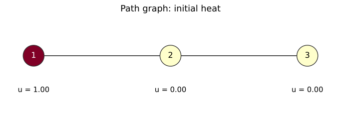
G = nx.path_graph([1, 2, 3])
L = nx.laplacian_matrix(G, nodelist=[1, 2, 3]).toarray().astype(float)
u0 = np.array([1, 0, 0], dtype=float)
print('Laplacian:')
pprint(L)
show_math(r'\mathbf{L}=\begin{pmatrix}1&-1&0\\-1&2&-1\\0&-1&1\end{pmatrix},'
          r'\qquad\mathbf{u}_0=\begin{pmatrix}1\\0\\0\end{pmatrix}')

fig, ax = plt.subplots(figsize=(7, 2.50), layout='constrained')
positions = {1: (0, 0), 2: (1, 0), 3: (2, 0)}
nx.draw_networkx(G, positions, ax=ax, node_color=u0, cmap='YlOrRd',
                 vmin=0, vmax=1, node_size=1000, edgecolors='#333333',
                 font_color={1: 'white', 2: 'black', 3: 'black'})
for node, value in zip(G.nodes, u0):
    ax.text(positions[node][0], -0.0900, f'u = {sig3(value)}', ha='center')
ax.set_ylim(-0.160, 0.100)
ax.set_title('Path graph: initial heat')
ax.axis('off')
save_svg(fig, '01_path_graph.svg')
$$\frac{d\mathbf{u}}{dt}=-\mathbf{L}\mathbf{u},\qquad\mathbf{u}(0)=\mathbf{u}_0$$
Laplacian:
array([[1.00, -1.00, 0.00],
       [-1.00, 2.00, -1.00],
       [0.00, -1.00, 1.00]])
$$\mathbf{L}=\begin{pmatrix}1&-1&0\\-1&2&-1\\0&-1&1\end{pmatrix},\qquad\mathbf{u}_0=\begin{pmatrix}1\\0\\0\end{pmatrix}$$
2. Deriving the heat kernel
Define the matrix exponential by its series and differentiate term by term. In finite dimensions, both the series and its derivative series converge uniformly on bounded time intervals.
$$ \begin{aligned} \mathbf{H}_t&=e^{-t\mathbf{L}} =\sum_{m=0}^{\infty}\frac{(-t)^m}{m!}\mathbf{L}^m,\\ \frac{d\mathbf{H}_t}{dt} &=\sum_{m=1}^{\infty}\frac{m(-1)^m t^{m-1}}{m!}\mathbf{L}^m\\ &=-\mathbf{L}\sum_{r=0}^{\infty}\frac{(-t)^r}{r!}\mathbf{L}^r =-\mathbf{L}\mathbf{H}_t. \end{aligned} $$
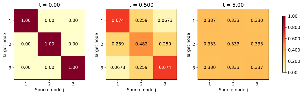
At $t=0$, only the $m=0$ term remains, giving $\mathbf{H}_0=\mathbf{I}$. Thus, the following expression solves the initial-value problem. The matrix $\mathbf{H}_t$ is called the heat kernel. Its $(i,j)$ entry is the heat at vertex $i$ when one unit of heat is initially placed at vertex $j$.
show_math(r'\boxed{\mathbf{u}(t)=\mathbf{H}_t\mathbf{u}_0'
          r'=e^{-t\mathbf{L}}\mathbf{u}_0}')

# np.exp acts entry by entry; use expm for a matrix exponential.
H1 = expm(-L)
print('H(1):')
pprint(H1)
print('u(1):')
pprint(H1 @ u0)
$$\boxed{\mathbf{u}(t)=\mathbf{H}_t\mathbf{u}_0=e^{-t\mathbf{L}}\mathbf{u}_0}$$
H(1):
array([[0.526, 0.317, 0.158],
       [0.317, 0.367, 0.317],
       [0.158, 0.317, 0.526]])
u(1):
array([0.526, 0.317, 0.158])
3. A three-vertex hand calculation
Find the eigenvalues from the characteristic equation. Expanding the determinant along the first row gives
$$ \begin{aligned} \det(\lambda\mathbf{I}-\mathbf{L}) &=(\lambda-1)\{(\lambda-2)(\lambda-1)-1\}-(\lambda-1)\\ &=(\lambda-1)(\lambda^2-3\lambda) =\lambda(\lambda-1)(\lambda-3). \end{aligned} $$
The eigenvalues are $0,1,3$. Substituting into $\mathbf{L}\mathbf{q}=\lambda\mathbf{q}$, for $\lambda=0$ all three components are equal. For $\lambda=1$, the second component is zero and the third is the negative of the first. For $\lambda=3$, the second component is $-2$ times the first, and the third equals the first. Normalizing each vector to length one gives
show_math(r'\mathbf{q}_0=\frac{1}{\sqrt{3}}\begin{pmatrix}1\\1\\1\end{pmatrix},'
          r'\quad\mathbf{q}_1=\frac{1}{\sqrt{2}}\begin{pmatrix}1\\0\\-1\end{pmatrix},'
          r'\quad\mathbf{q}_2=\frac{1}{\sqrt{6}}\begin{pmatrix}1\\-2\\1\end{pmatrix}')
show_math(r'\mathbf{q}_0^{\mathsf T}\mathbf{u}_0=\frac{1}{\sqrt{3}},'
          r'\quad\mathbf{q}_1^{\mathsf T}\mathbf{u}_0=\frac{1}{\sqrt{2}},'
          r'\quad\mathbf{q}_2^{\mathsf T}\mathbf{u}_0=\frac{1}{\sqrt{6}}')
$$\mathbf{q}_0=\frac{1}{\sqrt{3}}\begin{pmatrix}1\\1\\1\end{pmatrix},\quad\mathbf{q}_1=\frac{1}{\sqrt{2}}\begin{pmatrix}1\\0\\-1\end{pmatrix},\quad\mathbf{q}_2=\frac{1}{\sqrt{6}}\begin{pmatrix}1\\-2\\1\end{pmatrix}$$
$$\mathbf{q}_0^{\mathsf T}\mathbf{u}_0=\frac{1}{\sqrt{3}},\quad\mathbf{q}_1^{\mathsf T}\mathbf{u}_0=\frac{1}{\sqrt{2}},\quad\mathbf{q}_2^{\mathsf T}\mathbf{u}_0=\frac{1}{\sqrt{6}}$$
Decompose the initial values into orthogonal eigenvectors. Each coefficient satisfies $dc_k/dt=-\lambda_kc_k$. Since $d(e^{\lambda_kt}c_k)/dt=0$, we have $c_k(t)=e^{-\lambda_kt}c_k(0)$. Reconstruct the vector by adding the contributions component by component.
show_math(r'\begin{aligned}'
          r'\mathbf{u}(t)&=\sum_{k=0}^{2}e^{-\lambda_k t}'
          r'\mathbf{q}_k(\mathbf{q}_k^{\mathsf T}\mathbf{u}_0)\\'
          r'&=\frac{1}{3}\begin{pmatrix}1\\1\\1\end{pmatrix}'
          r'+\frac{e^{-t}}{2}\begin{pmatrix}1\\0\\-1\end{pmatrix}'
          r'+\frac{e^{-3t}}{6}\begin{pmatrix}1\\-2\\1\end{pmatrix}\\'
          r'&=\begin{pmatrix}\frac13+\frac12e^{-t}+\frac16e^{-3t}\\'
          r'\frac13-\frac13e^{-3t}\\'
          r'\frac13-\frac12e^{-t}+\frac16e^{-3t}\end{pmatrix}'
          r'\end{aligned}')

times = np.linspace(0, 6, 181)
heat = np.array([expm(-t * L) @ u0 for t in times])
analytical = np.column_stack([
    1 / 3 + np.exp(-times) / 2 + np.exp(-3 * times) / 6,
    1 / 3 - np.exp(-3 * times) / 3,
    1 / 3 - np.exp(-times) / 2 + np.exp(-3 * times) / 6,
])
np.testing.assert_allclose(heat, analytical, atol=1.00e-13)
pprint({'maximum error between hand calculation and expm': sig3(np.max(np.abs(heat - analytical)))})

fig, ax = plt.subplots(figsize=(7, 4), layout='constrained')
for i in range(3):
    ax.plot(times, heat[:, i], label=f'node {i + 1}')
ax.axhline(1 / 3, color='black', linestyle='--', label='limit = 1/3')
ax.set(xlabel='Time t', ylabel='Heat', title='Diffusion on three nodes')
format_axes(ax)
ax.legend()
save_svg(fig, '02_path_diffusion.svg')
$$\begin{aligned}\mathbf{u}(t)&=\sum_{k=0}^{2}e^{-\lambda_k t}\mathbf{q}_k(\mathbf{q}_k^{\mathsf T}\mathbf{u}_0)\\&=\frac{1}{3}\begin{pmatrix}1\\1\\1\end{pmatrix}+\frac{e^{-t}}{2}\begin{pmatrix}1\\0\\-1\end{pmatrix}+\frac{e^{-3t}}{6}\begin{pmatrix}1\\-2\\1\end{pmatrix}\\&=\begin{pmatrix}\frac13+\frac12e^{-t}+\frac16e^{-3t}\\\frac13-\frac13e^{-3t}\\\frac13-\frac12e^{-t}+\frac16e^{-3t}\end{pmatrix}\end{aligned}$$
{'maximum error between hand calculation and expm': '3.11e-15'}
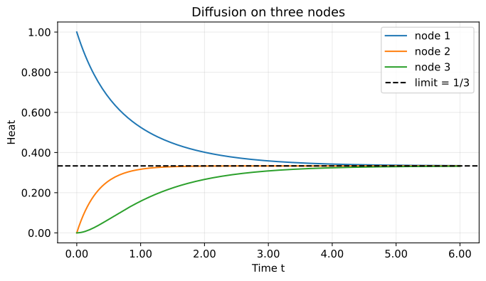
At $t=1$, the heat values are $0.526,0.317,0.158$, in order. Their displayed sum differs from exactly one because of rounding. Setting $t=0$ in the derived formula recovers the initial value $(1,0,0)^{\mathsf T}$, and the three components sum to one at every time.
The next figure shows the heat kernel itself. Columns indicate heat sources and rows indicate the observed vertices. As time passes, every column approaches a uniform distribution.
fig, axes = plt.subplots(1, 3, figsize=(11, 3.30), layout='constrained')
for ax, t in zip(axes, [0, 0.500, 5.00]):
    H = expm(-t * L)
    im = ax.imshow(H, cmap='YlOrRd', vmin=0, vmax=1)
    for i in range(3):
        for j in range(3):
            color = 'white' if H[i, j] > 0.600 else 'black'
            ax.text(j, i, sig3(H[i, j]), ha='center', va='center', color=color)
    ax.set(xticks=range(3), xticklabels=[1, 2, 3],
           yticks=range(3), yticklabels=[1, 2, 3],
           xlabel='Source node j', ylabel='Target node i', title=f't = {sig3(t)}')
cbar = fig.colorbar(im, ax=axes, shrink=0.800)
cbar.ax.yaxis.set_major_formatter(FuncFormatter(lambda x, _: sig3(x)))
save_svg(fig, '03_heat_kernels.svg')
4. Conservation and the role of eigenvalues
Let $\mathbf{1}$ be the all-ones vector. Zero row sums give $\mathbf{L}\mathbf{1}=\mathbf{0}$, and symmetry implies that total heat is conserved.
$$ \frac{d}{dt}(\mathbf{1}^{\mathsf T}\mathbf{u}) =-\mathbf{1}^{\mathsf T}\mathbf{L}\mathbf{u}=0. $$
Also, set $a=\max_i d_i>0$ and $\mathbf{P}=\mathbf{I}-\mathbf{L}/a$. Every entry of $\mathbf{P}$ is nonnegative.
$$ \mathbf{H}_t=e^{at(\mathbf{P}-\mathbf{I})} =e^{-at}\sum_{m=0}^{\infty}\frac{(at)^m}{m!}\mathbf{P}^m. $$
Thus, $\mathbf{H}_t$ is nonnegative for $t\geq0$, and nonnegative initial values remain nonnegative. If the total is one, the solution can also be viewed as the probability distribution of a continuous-time random walk with edge transition rates $w_{ij}$.
Nonnegative eigenvalues follow from the next calculation for any real vector $\mathbf{x}$.
$$ \begin{aligned} \mathbf{x}^{\mathsf T}\mathbf{L}\mathbf{x} &=\sum_i d_ix_i^2-\sum_{i,j}w_{ij}x_ix_j\\ &=\frac12\sum_{i,j}w_{ij}(x_i^2+x_j^2-2x_ix_j)\\ &=\frac12\sum_{i,j}w_{ij}(x_i-x_j)^2\geq0. \end{aligned} $$
For a connected graph, equality holds only when all components are equal. Order the eigenvalues as $0=\lambda_0<\lambda_1\leq\cdots$ and let $\mathbf{q}_k$ be orthonormal eigenvectors. Only $\mathbf{q}_0=\mathbf{1}/\sqrt{n}$ remains without decay.
show_math(r'\mathbf{H}_t=\sum_{k=0}^{n-1}e^{-t\lambda_k}'
          r'\mathbf{q}_k\mathbf{q}_k^{\mathsf T},\qquad'
          r'\lim_{t\to\infty}\mathbf{H}_t='
          r'\frac{\mathbf{1}\mathbf{1}^{\mathsf T}}{n}')
show_math(r'\mathbf{u}_{\infty}=\bar{u}\mathbf{1},\qquad'
          r'\bar{u}=\frac{\mathbf{1}^{\mathsf T}\mathbf{u}_0}{n}')

# Compare the eigendecomposition calculation with the matrix exponential.
eigenvalues, Q = eigh(L)
H_spectral = (Q * np.exp(-eigenvalues)) @ Q.T
np.testing.assert_allclose(H1, H_spectral, atol=1.00e-13)
np.testing.assert_allclose(H1.sum(axis=0), np.ones(3), atol=1.00e-13)
np.testing.assert_allclose(H1.sum(axis=1), np.ones(3), atol=1.00e-13)
assert H1.min() >= -1.00e-14
np.testing.assert_allclose(expm(-2 * L), H1 @ H1, atol=1.00e-13)
pprint({'maximum total-heat error': sig3(np.max(np.abs(heat.sum(axis=1) - 1))),
        'maximum eigendecomposition difference': sig3(np.max(np.abs(H1 - H_spectral)))})

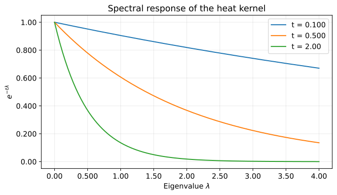
# Components with larger eigenvalues decay faster.
lam = np.linspace(0, 4, 200)
fig, ax = plt.subplots(figsize=(7, 4), layout='constrained')
for t in [0.100, 0.500, 2.00]:
    ax.plot(lam, np.exp(-t * lam), label=f't = {sig3(t)}')
ax.set(xlabel=r'Eigenvalue $\lambda$', ylabel=r'$e^{-t\lambda}$',
       title='Spectral response of the heat kernel')
format_axes(ax)
ax.legend()
save_svg(fig, '04_spectral_response.svg')
$$\mathbf{H}_t=\sum_{k=0}^{n-1}e^{-t\lambda_k}\mathbf{q}_k\mathbf{q}_k^{\mathsf T},\qquad\lim_{t\to\infty}\mathbf{H}_t=\frac{\mathbf{1}\mathbf{1}^{\mathsf T}}{n}$$
$$\mathbf{u}_{\infty}=\bar{u}\mathbf{1},\qquad\bar{u}=\frac{\mathbf{1}^{\mathsf T}\mathbf{u}_0}{n}$$
{'maximum eigendecomposition difference': '2.89e-15', 'maximum total-heat error': '1.78e-15'}
If the graph is disconnected, heat cannot move between connected components, and each component approaches its own mean. The uniform limit here comes from the combinatorial Laplacian. A different walk that gives each vertex a total outgoing transition rate of one has a stationary distribution proportional to degree.
5. Weak connections and diffusion speed
Let $c_k=\mathbf{q}_k^{\mathsf T}\mathbf{u}_0$ be the initial coefficients of the deviation from the mean. Orthonormality gives
$$ \begin{aligned} \|\mathbf{u}(t)-\bar{u}\mathbf{1}\|_2^2 &=\sum_{k=1}^{n-1}e^{-2t\lambda_k}c_k^2\\ &\leq e^{-2t\lambda_1}\sum_{k=1}^{n-1}c_k^2\\ &=e^{-2t\lambda_1}\|\mathbf{u}_0-\bar{u}\mathbf{1}\|_2^2. \end{aligned} $$
Taking square roots bounds the distance by $e^{-t\lambda_1}$ times its initial value. The eigenvalue $\lambda_1$ is the spectral gap. Decay is faster if the initial values contain no component in its eigendirection.
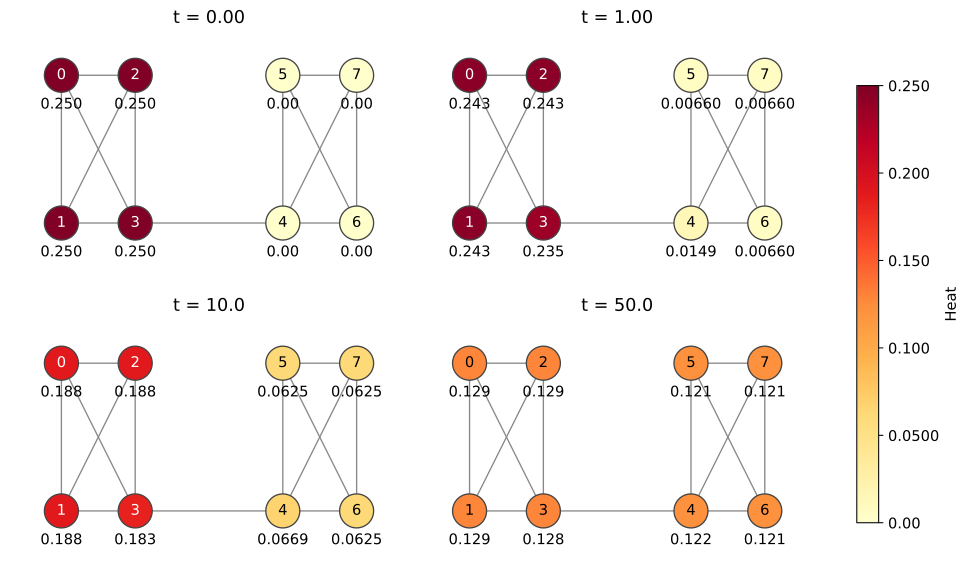
Join two complete graphs of four vertices each with a single edge. Internal edges have weight one, and the bridge has weight $w$. Place $1/4$ units of heat at each vertex in the left group. First examine $w=0.150$. For sparse matrices, expm_multiply applies the heat kernel to a vector without forming the full dense kernel.
def bridge_graph(weight):
    """Connect two complete graphs with a weighted bridge."""
    graph = nx.disjoint_union(nx.complete_graph(4), nx.complete_graph(4))
    nx.set_edge_attributes(graph, 1, 'weight')
    graph.add_edge(3, 4, weight=weight)
    return graph


bridge = bridge_graph(0.150)
L_bridge = nx.laplacian_matrix(bridge, nodelist=range(8)).astype(float)
initial = np.array([1, 1, 1, 1, 0, 0, 0, 0], dtype=float) / 4
steady = np.ones(8) / 8
positions = {0: (-2, 1), 1: (-2, -1), 2: (-1, 1), 3: (-1, -1),
             4: (1, -1), 5: (1, 1), 6: (2, -1), 7: (2, 1)}

fig, axes = plt.subplots(2, 2, figsize=(10, 6), layout='constrained')
for ax, t in zip(axes.flat, [0, 1, 10, 50]):
    values = expm_multiply(-t * L_bridge, initial)
    nx.draw_networkx_edges(bridge, positions, ax=ax, edge_color='#888888')
    nodes = nx.draw_networkx_nodes(
        bridge, positions, ax=ax, node_color=values, cmap='YlOrRd',
        vmin=0, vmax=0.250, node_size=650, edgecolors='#444444',
    )
    # Show numbers as well as colors and use the same scale to compare times.
    for node, (x, y) in positions.items():
        ax.text(x, y, str(node), ha='center', va='center',
                color='white' if values[node] > 0.150 else 'black')
        ax.text(x, y - 0.450, sig3(values[node]), ha='center')
    ax.set_title(f't = {sig3(t)}')
    ax.set(xlim=(-2.70, 2.70), ylim=(-1.90, 1.60))
    ax.axis('off')
cbar = fig.colorbar(nodes, ax=list(axes.flat), shrink=0.800, label='Heat')
cbar.ax.yaxis.set_major_formatter(FuncFormatter(lambda x, _: sig3(x)))
save_svg(fig, '05_bridge_diffusion.svg')
Next, vary only the bridge weight. Solid lines show distance from the mean, and dashed lines show the bound derived above. For this initial value, the two are close and nearly overlap. A smaller bridge weight gives a smaller gap, so the heat difference between the groups persists longer.
grid = np.linspace(0, 80, 161)
initial_distance = np.linalg.norm(initial - steady)
fig, ax = plt.subplots(figsize=(8, 4.50), layout='constrained')
report = []
for weight, color in zip([0.0500, 0.200, 1.00], ['#0072B2', '#D55E00', '#009E73']):
    graph = bridge_graph(weight)
    sparse_L = nx.laplacian_matrix(graph, nodelist=range(8)).astype(float)
    gap = eigh(sparse_L.toarray(), eigvals_only=True)[1]
    # Compute several equally spaced times together.
    trajectory = expm_multiply(-sparse_L, initial, start=0, stop=80, num=len(grid))
    distance = np.linalg.norm(trajectory - steady, axis=1)
    bound = initial_distance * np.exp(-gap * grid)
    ax.semilogy(grid, distance, color=color,
                label=f'w = {sig3(weight)}, gap = {sig3(gap)}')
    ax.semilogy(grid, bound, '--', color=color, alpha=0.650)

    # Check conservation, nonnegativity, the decay bound, and agreement with another calculation method.
    np.testing.assert_allclose(trajectory.sum(axis=1), np.ones(len(grid)), atol=1.00e-12)
    assert trajectory.min() >= -1.00e-12
    assert np.all(distance <= bound + 1.00e-12)
    np.testing.assert_allclose(
        trajectory[10], expm(-grid[10] * sparse_L.toarray()) @ initial, atol=1.00e-12,
    )
    report.append({'bridge weight': sig3(weight), 'gap': sig3(gap),
                   'distance at time 80': sig3(distance[-1])})

ax.set(xlabel='Time t', ylabel='Distance from the mean',
       title='Solid: distance / dashed: spectral bound')
format_axes(ax)
ax.yaxis.set_minor_formatter(matplotlib.ticker.NullFormatter())
ax.legend()
save_svg(fig, '06_bridge_mixing.svg')
pprint(report, sort_dicts=False)
print('Checked the hand calculation, conservation, nonnegativity, semigroup property, and decay bound.')
print(f'SVG saved to: {OUT}')
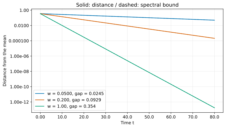
[{'bridge weight': '0.0500', 'gap': '0.0245', 'distance at time 80': '0.0497'},
 {'bridge weight': '0.200', 'gap': '0.0929', 'distance at time 80': '0.000210'},
 {'bridge weight': '1.00', 'gap': '0.354', 'distance at time 80': '1.72e-13'}]
Checked the hand calculation, conservation, nonnegativity, semigroup property, and decay bound.
SVG saved to: 106_nb_files
Conclusion
We represented graph diffusion with a heat kernel and checked heat conservation, convergence to the mean, and eigenvalue-dependent decay by hand and in Python.
On a connected undirected graph, diffusion with the combinatorial Laplacian approaches the mean of the initial values. Weak connections create a small spectral gap and slow diffusion between groups. Use expm for small examples and expm_multiply when only the distribution is needed on a sparse graph.