What does least squares do in physics, statistics, and machine learning? (Rewritten from an earlier blog post)
Environment
Python 3.14.6, NumPy 2.5.4, Matplotlib 3.11.2 (Jupyter Notebook).
This article is a rewrite of a post from around 2013–2016, with calculations performed in the environment described above.
Overview
Least squares minimizes the sum of squared differences between observations and a model. In physics, it estimates constants from measurements; in statistics, it estimates parameters under assumptions about errors; in machine learning, it fits prediction models. We derive the shared calculation and compare spring measurements with polynomial regression in Python. All data are generated artificially.
Setup
Run the code in Jupyter Notebook from top to bottom. Round numbers to three significant digits only when displaying them.
import platform
from pathlib import Path
from pprint import pprint

import matplotlib
import matplotlib.pyplot as plt
import numpy as np
from IPython.display import Latex, display
from matplotlib.ticker import FuncFormatter, LogLocator, NullFormatter
from matplotlib_inline.backend_inline import set_matplotlib_formats

%matplotlib inline
set_matplotlib_formats("svg")

print("Python:", platform.python_version())
pprint({"NumPy": np.__version__, "Matplotlib": matplotlib.__version__})

# Use the same number of significant digits for arrays, axis ticks, and decimals in formulas.
def sig3(value):
    return f"{float(value):#.3g}"


def tex3(value):
    parts = sig3(value).split("e")
    if len(parts) == 1:
        return parts[0]
    return parts[0] + rf"\times 10^{{{int(parts[1])}}}"


def show_formula(formula):
    # Enclose key formulas in \( ... \) and render them as LaTeX.
    display(Latex(r"\(\displaystyle " + formula + r"\)"))


np.set_printoptions(formatter={"float_kind": sig3})
plt.rcParams.update({"font.size": 11, "svg.fonttype": "none"})
figure_dir = Path("101_nb_files")
figure_dir.mkdir(exist_ok=True)


def save_figure(fig, filename):
    """Format tick labels and retain figures both as SVG files and in the notebook."""
    for ax in fig.axes:
        if ax.get_xscale() == "log":
            ax.xaxis.set_major_locator(LogLocator(base=10, numticks=5))
        if ax.get_yscale() == "log":
            ax.yaxis.set_major_locator(LogLocator(base=10, subs=(1, 2, 5)))
        for axis in (ax.xaxis, ax.yaxis):
            axis.set_major_formatter(FuncFormatter(lambda value, pos: sig3(value)))
            axis.set_minor_formatter(NullFormatter())
        ax.grid(True, alpha=0.250)
    fig.tight_layout()
    fig.savefig(figure_dir / filename, format="svg", bbox_inches="tight")
    plt.show()
    plt.close(fig)
Python: 3.14.6
{'Matplotlib': '3.11.2', 'NumPy': '2.5.4'}
1. The shared calculation
Let $\mathbf{y}$ contain the observations, $\mathbf{b}$ the coefficients, and $\mathbf{X}$ the explanatory variables. Minimize the sum of squares of the residuals $\mathbf{r}=\mathbf{y}-\mathbf{X}\mathbf{b}$.
$$ \begin{aligned} S(\mathbf{b}) &=(\mathbf{y}-\mathbf{X}\mathbf{b})^{\mathsf T}(\mathbf{y}-\mathbf{X}\mathbf{b})\\ &=\mathbf{y}^{\mathsf T}\mathbf{y}-2\mathbf{b}^{\mathsf T}\mathbf{X}^{\mathsf T}\mathbf{y} +\mathbf{b}^{\mathsf T}\mathbf{X}^{\mathsf T}\mathbf{X}\mathbf{b},\\ \nabla_{\mathbf{b}}S &=-2\mathbf{X}^{\mathsf T}\mathbf{y}+2\mathbf{X}^{\mathsf T}\mathbf{X}\mathbf{b}=\mathbf{0},\\ \mathbf{X}^{\mathsf T}\mathbf{X}\hat{\mathbf{b}}&=\mathbf{X}^{\mathsf T}\mathbf{y}. \end{aligned} $$
If the columns of $\mathbf{X}$ are linearly independent, $\mathbf{X}^{\mathsf T}\mathbf{X}$ is positive definite and the solution is unique.
show_formula(
    r"\hat{\mathbf{b}}=(\mathbf{X}^{\mathsf T}\mathbf{X})^{-1}"
    r"\mathbf{X}^{\mathsf T}\mathbf{y}"
)
$$ \displaystyle \hat{\mathbf{b}}=(\mathbf{X}^{\mathsf T}\mathbf{X})^{-1}\mathbf{X}^{\mathsf T}\mathbf{y} $$
We also have $\mathbf{X}^{\mathsf T}\hat{\mathbf{r}}=\mathbf{X}^{\mathsf T}\mathbf{y}-\mathbf{X}^{\mathsf T}\mathbf{X}\hat{\mathbf{b}}=\mathbf{0}$. The fitted values are the orthogonal projection of $\mathbf{y}$ onto the column space of $\mathbf{X}$. Use np.linalg.lstsq instead of forming an inverse. This function returns a minimum-norm solution even when the matrix is rank deficient; see the NumPy documentation.
2. Physics: estimating a spring constant from measurements
Write the external force stretching a spring as $F_i=c+kx_i+\varepsilon_i$. Here, $x_i$ is the extension, $k$ the spring constant, and $c$ the zero offset in the force measurement. Ignore errors in extension and work within the range where Hooke’s law applies. Row $i$ of $\mathbf{X}$ is $(1,x_i)$, and $\mathbf{b}=(c,k)^{\mathsf T}$.
$$ \begin{aligned} S(c,k)&=\sum_i(F_i-c-kx_i)^2,\\ \frac{\partial S}{\partial c}&=-2\sum_i(F_i-c-kx_i)=0\\ &\Rightarrow\hat c=\bar F-\hat k\bar x,\\ \frac{\partial S}{\partial k}&=-2\sum_i x_i(F_i-c-kx_i)=0\\ &\Rightarrow\sum_i x_iF_i=(\bar F-\hat k\bar x)\sum_i x_i+\hat k\sum_i x_i^2\\ &=n\bar x\bar F+\hat k(\sum_i x_i^2-n\bar x^2),\\ \hat k&=\frac{\sum_i x_iF_i-n\bar x\bar F}{\sum_i x_i^2-n\bar x^2}. \end{aligned} $$
Bars denote sample means. If every extension is the same, the denominator is zero and $c$ and $k$ cannot be estimated separately.
# Control extension exactly and add independent normal errors only to force measurements.
rng_physics = np.random.default_rng(101)
x = np.linspace(0, 0.100, 20)
sigma = 0.0300 + 0.900 * x  # Known standard deviation of each measurement [N]
X = np.column_stack((np.ones(x.size), x))
b_true = np.array([0.100, 20.0])  # c [N], k [N/m]
force = X @ b_true + rng_physics.normal(0, sigma)
b_ols = np.linalg.lstsq(X, force, rcond=None)[0]
residual_ols = force - X @ b_ols

# Also check that the hand-derived formulas agree with the matrix solution.
k_manual = ((x - x.mean()) @ (force - force.mean())) / np.sum((x - x.mean()) ** 2)
c_manual = force.mean() - k_manual * x.mean()
assert np.allclose(b_ols, [c_manual, k_manual])
assert np.allclose(X.T @ residual_ols, 0, atol=1.00e-12)
pprint({"true values [c, k]": b_true, "ordinary least squares [c, k]": b_ols})
show_formula(rf"\hat F(x)={tex3(b_ols[0])}+{tex3(b_ols[1])}x")

fig, ax = plt.subplots(figsize=(7.20, 4.50))
ax.scatter(x, force, color="tab:blue", label="Measurements", zorder=3)
ax.plot(x, X @ b_true, "--", color="black", label="True relation")
ax.plot(x, X @ b_ols, color="tab:orange", label="OLS")
ax.vlines(x, X @ b_ols, force, color="tab:gray", alpha=0.700, label="Residuals")
ax.set(xlabel="Extension x [m]", ylabel="Force F [N]", title="1. Fitting a physical parameter")
ax.legend()
save_figure(fig, "01_spring_ols.svg")

# Plot contours of the sum of squares as the intercept and slope vary.
c_grid = np.linspace(b_ols[0] - 0.120, b_ols[0] + 0.120, 101)
k_grid = np.linspace(b_ols[1] - 3, b_ols[1] + 3, 101)
C, K = np.meshgrid(c_grid, k_grid)
loss_grid = np.sum((force[:, None, None] - C - x[:, None, None] * K) ** 2, axis=0)
fig, ax = plt.subplots(figsize=(7.20, 4.50))
contours = ax.contour(C, K, loss_grid, levels=9, cmap="viridis")
ax.clabel(contours, fmt=lambda value: sig3(value))
ax.plot(*b_ols, "o", color="tab:red", label="OLS minimum")
ax.set(xlabel="Offset c [N]", ylabel="Spring constant k [N/m]", title="2. Residual sum of squares [N squared]")
ax.legend()
save_figure(fig, "02_loss_contours.svg")
{'true values [c, k]': array([0.100, 20.0]), 'ordinary least squares [c, k]': array([0.123, 19.4])}
$$ \displaystyle \hat F(x)=0.123+19.4x $$
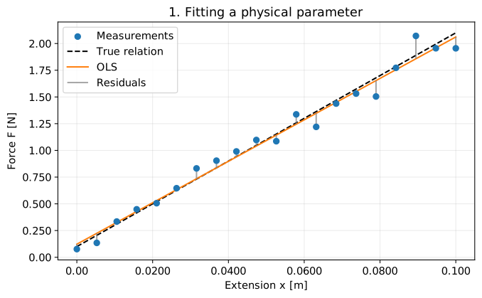
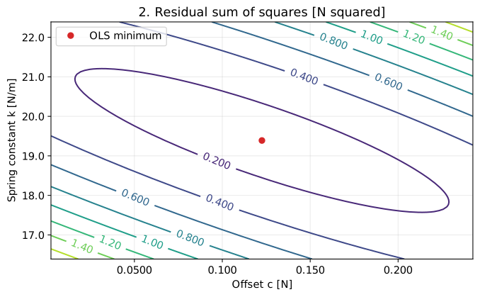
The vertical lines in Figure 1 are residuals, and their squared lengths are added. The tilt of the ellipses in Figure 2 shows how changes in the intercept and slope can offset each other.
If the standard deviation $\sigma_i$ of each measurement is known, weights can account for differences in precision. Weighted least squares minimizes
$$ S_w=\sum_i\left(\frac{F_i-c-kx_i}{\sigma_i}\right)^2 =\|\widetilde{\mathbf{y}}-\widetilde{\mathbf{X}}\mathbf{b}\|_2^2, \quad \widetilde y_i=F_i/\sigma_i,\quad \widetilde X_{ij}=X_{ij}/\sigma_i $$
The weights are $1/\sigma_i^2$. The error bars below show $\pm\sigma_i$. The weighted estimate is closer to the true value in this example, but this is not guaranteed every time.
# Divide each row by its standard deviation and use the same least-squares solver.
X_white = X / sigma[:, None]
force_white = force / sigma
b_wls = np.linalg.lstsq(X_white, force_white, rcond=None)[0]
residual_wls = force - X @ b_wls
assert np.allclose(X_white.T @ (residual_wls / sigma), 0, atol=1.00e-10)
pprint({"weighted [c, k]": b_wls, "weighted sum of squares": sig3(np.sum((residual_wls / sigma) ** 2))})

fig, axes = plt.subplots(1, 2, figsize=(10.0, 4.20))
axes[0].errorbar(x, force, yerr=sigma, fmt="o", markersize=4, capsize=3, label="Measurements")
axes[0].plot(x, X @ b_true, "--", color="black", label="True relation")
axes[0].plot(x, X @ b_ols, label="OLS")
axes[0].plot(x, X @ b_wls, label="WLS")
axes[0].set(xlabel="Extension x [m]", ylabel="Force F [N]", title="3a. Known measurement uncertainty")
axes[0].legend()
axes[1].axhline(0, color="black", linewidth=1)
axes[1].plot(x, residual_ols / sigma, "o-", label="OLS")
axes[1].plot(x, residual_wls / sigma, "s-", label="WLS")
axes[1].set(xlabel="Extension x [m]", ylabel=r"Residual / $\sigma_i$", title="3b. Standardized residuals")
axes[1].legend()
save_figure(fig, "03_weighted_fit_residuals.svg")
{'weighted [c, k]': array([0.0934, 20.1]), 'weighted sum of squares': '22.7'}
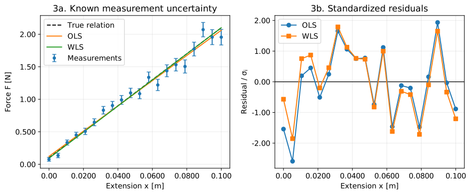
Plotting residuals against extension helps reveal whether deviations are concentrated in a particular range. Squaring residuals makes least squares sensitive to large outliers. Adding weights does not resolve systematic errors or extend the range where the physical law applies.
3. Statistics: maximum likelihood with normal errors
Assume independent errors $\varepsilon_i\sim\mathcal N(0,\sigma_i^2)$, with known $\sigma_i$. The likelihood is the product of the densities, and taking its logarithm turns the product into a sum.
$$ \begin{aligned} L(\mathbf{b})&=\prod_i\frac{1}{\sqrt{2\pi\sigma_i^2}} \exp\left[-\frac{(F_i-c-kx_i)^2}{2\sigma_i^2}\right],\\ \log L(\mathbf{b})&=-\frac12\sum_i\log(2\pi\sigma_i^2) -\frac12\sum_i\frac{(F_i-c-kx_i)^2}{\sigma_i^2},\\ -\log L(\mathbf{b})&=C+\frac12 S_w(\mathbf{b}). \end{aligned} $$
Here, $C$ is constant with respect to the coefficients. Maximizing the likelihood is equivalent to minimizing the weighted sum of squares. If all $\sigma_i$ are equal, this becomes ordinary least squares. The least-squares calculation itself, however, does not require a normality assumption.
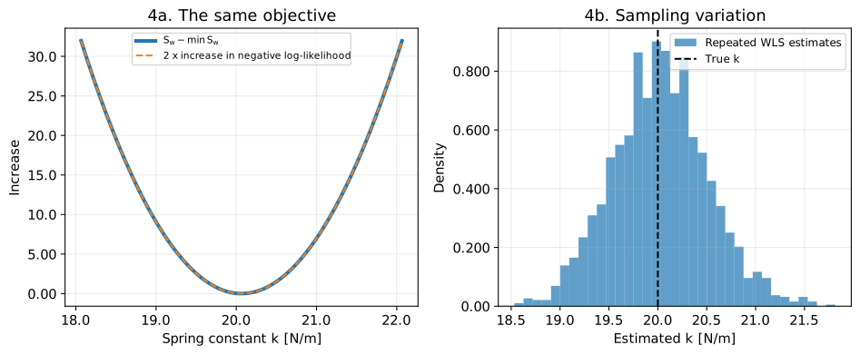
The left panel of Figure 4 fixes $c$ at its estimate and compares increases above the minimum. The right panel shows the distribution of $\hat k$ after generating the same measurement experiment 2,000 times. It reveals estimation variability that cannot be seen from a single fit.
k_scan = np.linspace(b_wls[1] - 2, b_wls[1] + 2, 201)
residual_scan = force[:, None] - (b_wls[0] + x[:, None] * k_scan)
weighted_scan = np.sum((residual_scan / sigma[:, None]) ** 2, axis=0)
nll = np.sum(np.log(np.sqrt(2 * np.pi) * sigma)) + weighted_scan / 2
delta_weighted = weighted_scan - weighted_scan.min()
delta_nll = 2 * (nll - nll.min())
assert np.allclose(delta_weighted, delta_nll)

# Treat each column as an independent experiment and estimate 2,000 coefficient sets together.
rng_repeat = np.random.default_rng(102)
repeats = 2000
force_repeated = X @ b_true[:, None] + rng_repeat.normal(
    0, sigma[:, None], size=(x.size, repeats)
)
b_repeated = np.linalg.lstsq(X_white, force_repeated / sigma[:, None], rcond=None)[0]
pprint({
    "mean k [N/m]": sig3(b_repeated[1].mean()),
    "standard deviation of k [N/m]": sig3(b_repeated[1].std(ddof=1)),
})

fig, axes = plt.subplots(1, 2, figsize=(10.0, 4.20))
axes[0].plot(k_scan, delta_weighted, linewidth=3, label=r"$S_w-\min S_w$")
axes[0].plot(k_scan, delta_nll, "--", label="2 x increase in negative log-likelihood")
axes[0].set(xlabel="Spring constant k [N/m]", ylabel="Increase", title="4a. The same objective")
axes[0].legend(fontsize=8)
axes[1].hist(b_repeated[1], bins=35, density=True, alpha=0.700, label="Repeated WLS estimates")
axes[1].axvline(b_true[1], color="black", linestyle="--", label="True k")
axes[1].set(xlabel="Estimated k [N/m]", ylabel="Density", title="4b. Sampling variation")
axes[1].legend(fontsize=9)
save_figure(fig, "04_likelihood_sampling.svg")
{'mean k [N/m]': '20.0', 'standard deviation of k [N/m]': '0.487'}
4. Machine learning: predicting unseen data
Regression uses $S/n$ as the mean squared error (MSE). Dividing by the constant $n$ does not change the minimizing coefficients. Here, approximate $y=\sin(\pi x)+\varepsilon$ by a degree-12 polynomial $\sum_{j=0}^{12}b_jx^j$. Although it is nonlinear in $x$, it is linear in the coefficients, so least squares applies.
Reducing training error alone can also fit the noise. Ridge regression adds a penalty on squared coefficients. Set $\mathbf{D}=\operatorname{diag}(0,1,\ldots,1)$ so that the intercept is not penalized.
$$ \begin{aligned} J(\mathbf{b})&=\frac1n\|\mathbf{y}-\mathbf{X}\mathbf{b}\|_2^2 +\lambda\|\mathbf{D}\mathbf{b}\|_2^2,\\ \nabla_{\mathbf{b}}J&=\frac2n(\mathbf{X}^{\mathsf T}\mathbf{X}\mathbf{b} -\mathbf{X}^{\mathsf T}\mathbf{y})+2\lambda\mathbf{D}^{\mathsf T}\mathbf{D}\mathbf{b}=\mathbf{0},\\ (\mathbf{X}^{\mathsf T}\mathbf{X}+n\lambda\mathbf{D}^{\mathsf T}\mathbf{D})\hat{\mathbf{b}} &=\mathbf{X}^{\mathsf T}\mathbf{y}. \end{aligned} $$
Implement this by appending $\sqrt{n\lambda}\mathbf{D}$ below $\mathbf{X}$ and zeros below $\mathbf{y}$. The resulting sum of squares is $S+n\lambda\|\mathbf{D}\mathbf{b}\|_2^2=nJ$.
Fit the coefficients on 18 training points and choose $\lambda$ using 100 independent validation points. Finally, evaluate on 1,000 test points that were not used for selection. All inputs lie in $[-1,1]$, and the noise standard deviation is $0.200$.
rng_ml = np.random.default_rng(2026)
x_train = np.linspace(-1, 1, 18)
x_valid = rng_ml.uniform(-1, 1, 100)
x_test = rng_ml.uniform(-1, 1, 1000)


def target(values):
    return np.sin(np.pi * values)


y_train = target(x_train) + rng_ml.normal(0, 0.200, x_train.size)
y_valid = target(x_valid) + rng_ml.normal(0, 0.200, x_valid.size)
y_test = target(x_test) + rng_ml.normal(0, 0.200, x_test.size)
degree = 12


def design(values):
    # Columns are ordered as 1, x, x**2, ..., x**12.
    return np.vander(values, N=degree + 1, increasing=True)


X_train, X_valid, X_test = (design(values) for values in (x_train, x_valid, x_test))
penalty = np.diag([0] + [1] * degree)


def fit_ridge(lam):
    # Multiply by n to match the penalty strength to the mean squared error defined in the text.
    augmented_X = np.vstack((X_train, np.sqrt(x_train.size * lam) * penalty))
    augmented_y = np.concatenate((y_train, np.zeros(degree + 1)))
    return np.linalg.lstsq(augmented_X, augmented_y, rcond=None)[0]


lambdas = np.logspace(-8, 0, 81)
coefficients = np.array([fit_ridge(lam) for lam in lambdas])
train_mse = np.mean((X_train @ coefficients.T - y_train[:, None]) ** 2, axis=0)
valid_mse = np.mean((X_valid @ coefficients.T - y_valid[:, None]) ** 2, axis=0)
best_index = np.argmin(valid_mse)  # Do not use test data for selection.
best_lambda = lambdas[best_index]
b_best = coefficients[best_index]
b_unregularized = fit_ridge(0)

show_formula(rf"\lambda_\ast={tex3(best_lambda)}")
rows = []
for name, coefficient in (("OLS", b_unregularized), ("Ridge", b_best)):
    rows.append({
        "model": name,
        "training MSE": sig3(np.mean((X_train @ coefficient - y_train) ** 2)),
        "validation MSE": sig3(np.mean((X_valid @ coefficient - y_valid) ** 2)),
        "test MSE": sig3(np.mean((X_test @ coefficient - y_test) ** 2)),
    })
pprint(rows, sort_dicts=False)

x_plot = np.linspace(-1, 1, 401)
X_plot = design(x_plot)
fig, ax = plt.subplots(figsize=(8.40, 4.80))
ax.scatter(x_train, y_train, color="black", s=25, label="Training data", zorder=4)
ax.plot(x_plot, target(x_plot), "--", color="black", label="True mean")
ax.plot(x_plot, X_plot @ b_unregularized, label="OLS (degree 12)", alpha=0.800)
ax.plot(x_plot, X_plot @ b_best, label="Ridge (validation choice)", linewidth=2)
ax.plot(x_plot, X_plot @ fit_ridge(1), label="Ridge (lambda = 1)", alpha=0.800)
ax.set(xlabel="Input x", ylabel="Target y", title="5. Prediction with and without regularization")
ax.legend(fontsize=9)
save_figure(fig, "05_prediction_curves.svg")

fig, ax = plt.subplots(figsize=(7.20, 4.50))
ax.loglog(lambdas, train_mse, label="Training MSE")
ax.loglog(lambdas, valid_mse, label="Validation MSE")
ax.axvline(best_lambda, color="black", linestyle="--", label="Selected lambda")
ax.set(xlabel=r"Regularization $\lambda$", ylabel="MSE", title="6. Choosing regularization on validation data")
ax.legend()
save_figure(fig, "06_validation_curve.svg")
$$ \displaystyle \lambda_\ast=6.31\times 10^{-5} $$
[{'model': 'OLS', 'training MSE': '0.0127', 'validation MSE': '0.0641', 'test MSE': '0.0764'},
 {'model': 'Ridge', 'training MSE': '0.0181', 'validation MSE': '0.0328', 'test MSE': '0.0432'}]
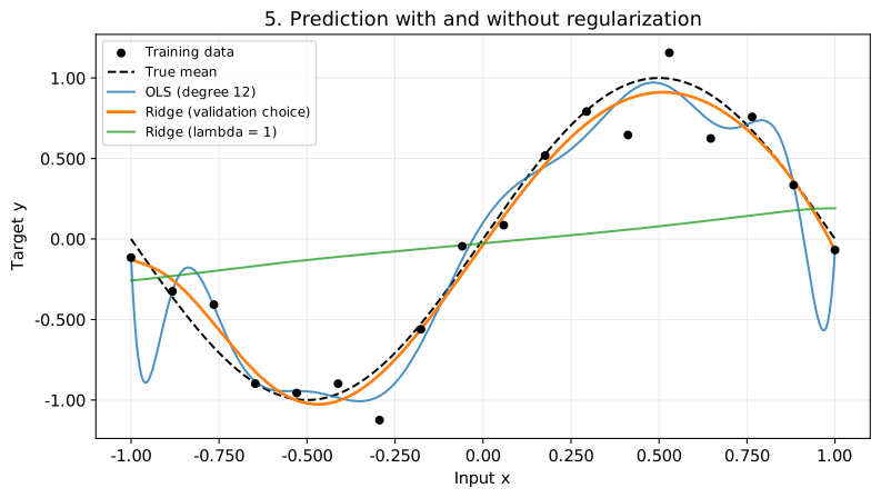
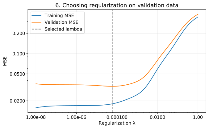
In this example, test MSE is $0.0764$ for ordinary least squares and $0.0432$ for Ridge. Excessive regularization prevents the curve from capturing peaks and troughs, as Figure 5 shows. In Figure 6, different regularization strengths minimize training and validation error. Results also depend on the sample and feature scales, so regularization does not always improve predictive accuracy.
Conclusion
We examined least squares in three roles: estimating physical constants, maximum-likelihood estimation in statistics, and regression in machine learning.
The shared calculation minimizes the residual sum of squares. Physics focuses on the law and measurement precision, statistics on the error distribution and estimation variability, and machine learning on errors for unseen data. Even with the same solver, the conditions needed to assess the result depend on its purpose.