Why do eigenvalue problems appear in PCA, vibrations, quantum mechanics, and graphs? (Rewritten from an earlier blog post)
Environment
Python 3.14.6, NumPy 2.5.4, SciPy 1.18.1, SymPy 1.14.0, Matplotlib 3.11.2 (Jupyter Notebook).
This article is a rewrite of a post from around 2013–2016, with calculations performed in the environment described above.
Overview
In an eigenvector basis, a matrix acts by scaling each component separately. Using symmetric or Hermitian matrices, we examine how PCA variance, vibration modes, quantum-state time evolution, and changes in graph vertex values lead to eigenvalue problems, and check them in Python.
Setup
Run the code in Jupyter Notebook from top to bottom. Round numbers to three significant digits only when displaying them.
import platform
from pathlib import Path
from pprint import pprint

import matplotlib
import matplotlib.pyplot as plt
import numpy as np
import scipy
import sympy as sp
from IPython.display import Math, display
from matplotlib.ticker import FuncFormatter
from matplotlib_inline.backend_inline import set_matplotlib_formats
from scipy.linalg import eigh

%matplotlib inline

print(f"Python: {platform.python_version()}")
print(f"NumPy: {np.__version__}, SciPy: {scipy.__version__}")
print(f"Matplotlib: {matplotlib.__version__}, SymPy: {sp.__version__}")

# Use three significant digits only for array and tick displays. Use English figure labels for portability.
np.set_printoptions(formatter={"float_kind": lambda value: f"{value:#.3g}"})
set_matplotlib_formats("svg")
plt.rcParams.update({
    "font.size": 11,
    "axes.grid": True,
    "grid.alpha": 0.200,
    "figure.figsize": (9, 4),
    "svg.fonttype": "none",
    "svg.hashsalt": "eigen-102",
})
figure_dir = Path("102_nb_files")
figure_dir.mkdir(parents=True, exist_ok=True)
colors = ["#2463a6", "#d05b30", "#2b856a"]


def save_figure(fig, name):
    """Format continuous tick labels, save as SVG, and display the figure."""
    for ax in fig.axes:
        for axis in (ax.xaxis, ax.yaxis):
            # Keep explicit category labels, such as principal-component numbers, unchanged.
            if not isinstance(axis.get_major_formatter(), FuncFormatter):
                axis.set_major_formatter(
                    FuncFormatter(lambda value, position: f"{value:#.3g}")
                )
    fig.savefig(figure_dir / name, format="svg", bbox_inches="tight",
                metadata={"Date": None})
    display(fig)
    plt.close(fig)
Python: 3.14.6
NumPy: 2.5.4, SciPy: 1.18.1
Matplotlib: 3.11.2, SymPy: 1.14.0
1. Decomposition into eigenvectors
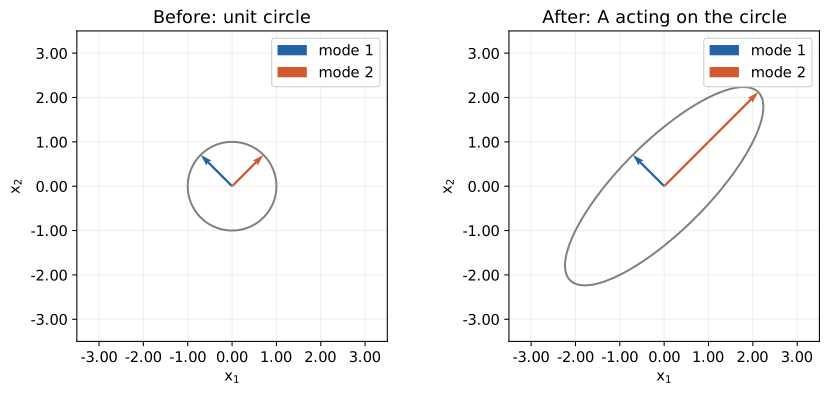
The equation $\mathbf{A}\mathbf{v}=\lambda\mathbf{v}$, with $\mathbf{v}\ne\mathbf{0}$, describes a direction that remains on the same line after the matrix acts. For a real symmetric matrix, let $\mathbf{Q}$ contain orthonormal eigenvectors as columns and $\mathbf{D}$ contain the eigenvalues on its diagonal. Then
$$ \begin{aligned} \mathbf{A}\mathbf{Q}&=\mathbf{Q}\mathbf{D},\quad \mathbf{Q}^{T}\mathbf{Q}=\mathbf{I},\\ \mathbf{A}&=\mathbf{Q}\mathbf{D}\mathbf{Q}^{T},\\ \mathbf{x}=\mathbf{Q}\mathbf{c} &\Longrightarrow\mathbf{Q}^{T}\mathbf{A}\mathbf{x}=\mathbf{D}\mathbf{c}. \end{aligned} $$
The next cell computes the characteristic equation of $\mathbf{A}=\begin{pmatrix}2&1\\1&2\end{pmatrix}$. Eigenvalue 3 gives $-v_1+v_2=0$, and eigenvalue 1 gives $v_1+v_2=0$. The normalized eigenvectors are $(1,1)^T/\sqrt2$ and $(1,-1)^T/\sqrt2$.
# Also check the characteristic polynomial symbolically.
lam = sp.Symbol("lambda")
A_exact = sp.Matrix([[2, 1], [1, 2]])
polynomial = (A_exact - lam * sp.eye(2)).det()
display(Math(r"\det(\mathbf{A}-\lambda\mathbf{I})=(2-\lambda)^2-1="
             + sp.latex(sp.expand(polynomial))
             + "=" + sp.latex(sp.factor(polynomial)) + "=0"))

A = np.array(A_exact, dtype=float)
values, vectors = np.linalg.eigh(A)
pprint({"eigenvalues": values, "eigenvectors (columns)": vectors})

# Overlay eigenvector directions on the unit circle and its transformed ellipse.
theta = np.linspace(0, 2 * np.pi, 361)
circle = np.array([np.cos(theta), np.sin(theta)])
fig, axes = plt.subplots(1, 2, figsize=(9, 4), layout="constrained")
for ax, points, scales, title in zip(
    axes, [circle, A @ circle], [np.ones(2), values],
    ["Before: unit circle", "After: A acting on the circle"],
):
    ax.plot(*points, color="0.500")
    for j in range(2):
        arrow = scales[j] * vectors[:, j]
        ax.quiver(0, 0, *arrow, angles="xy", scale_units="xy", scale=1,
                  color=colors[j], label=f"mode {j + 1}")
    ax.set(xlim=(-3.50, 3.50), ylim=(-3.50, 3.50),
           xlabel=r"$x_1$", ylabel=r"$x_2$", title=title)
    ax.set_aspect("equal")
    ax.legend()
save_figure(fig, "01_eigenvectors.svg")
$$ \displaystyle \det(\mathbf{A}-\lambda\mathbf{I})=(2-\lambda)^2-1=\lambda^{2} - 4 \lambda + 3=\left(\lambda - 3\right) \left(\lambda - 1\right)=0 $$
{'eigenvalues': array([1.00, 3.00]),
 'eigenvectors (columns)': array([[-0.707, 0.707],
       [0.707, 0.707]])}
2. PCA: maximizing variance
Let $\mathbf{X}\in\mathbb{R}^{n\times p}$ be data centered by subtracting each column mean, and let $\mathbf{v}$ be a unit direction. The projected values also have mean zero, so
$$ \mathbf{S}=\frac{\mathbf{X}^{T}\mathbf{X}}{n-1},\quad \mathbf{z}=\mathbf{X}\mathbf{v},\quad \frac{\mathbf{z}^{T}\mathbf{z}}{n-1} =\frac{\mathbf{v}^{T}\mathbf{X}^{T}\mathbf{X}\mathbf{v}}{n-1} =\mathbf{v}^{T}\mathbf{S}\mathbf{v}. $$
Adding the constraint $\mathbf{v}^{T}\mathbf{v}=1$ with a Lagrange multiplier gives
$$ \begin{aligned} F&=\mathbf{v}^{T}\mathbf{S}\mathbf{v}-\lambda(\mathbf{v}^{T}\mathbf{v}-1),\\ \nabla_{\mathbf{v}}F&=2\mathbf{S}\mathbf{v}-2\lambda\mathbf{v}=\mathbf{0}. \end{aligned} $$
$$\boxed{\mathbf{S}\mathbf{v}=\lambda\mathbf{v},\quad \mathbf{v}^{T}\mathbf{S}\mathbf{v}=\lambda}$$
The direction of the largest eigenvalue is the first principal component. Choose the remaining components in order from orthogonal directions. Here, the two variables use the same units. When scales differ, decide whether standardization is needed. MIT lecture on PCA
# Generate two correlated variables and subtract their sample means.
rng = np.random.default_rng(102)
X = rng.multivariate_normal([0, 0], [[2, 1], [1, 2]], size=400)
X -= X.mean(axis=0)
S = X.T @ X / (len(X) - 1)
pca_values, pca_vectors = np.linalg.eigh(S)
order = np.argsort(pca_values)[::-1]
pca_values, pca_vectors = pca_values[order], pca_vectors[:, order]
scores = X @ pca_vectors
explained = pca_values / pca_values.sum()
pprint({"sample covariance": S, "eigenvalues": pca_values,
        "explained variance ratio": explained})
display(Math(r"\operatorname{Var}(z_1)=" + f"{pca_values[0]:#.3g}"
             + r",\quad\operatorname{Var}(z_2)=" + f"{pca_values[1]:#.3g}"))
# In terms of eigenbasis coefficients a_i, the largest eigenvalue bounds the variance.
display(Math(r"\mathbf{v}=\mathbf{Q}\mathbf{a},\quad\sum_i a_i^2=1,\quad"
             r"\mathbf{v}^{T}\mathbf{S}\mathbf{v}=\sum_i\lambda_i a_i^2"
             r"\le\lambda_{\max}\sum_i a_i^2=\lambda_{\max}"))

fig, axes = plt.subplots(1, 2, figsize=(9, 4), layout="constrained")
axes[0].scatter(*X.T, s=10, alpha=0.350, color=colors[0])
for j in range(2):
    direction = 2 * np.sqrt(pca_values[j]) * pca_vectors[:, j]
    axes[0].plot([-direction[0], direction[0]],
                 [-direction[1], direction[1]], color=colors[j + 1],
                 lw=2, label=f"PC{j + 1}")
axes[0].set(xlabel=r"$x_1$", ylabel=r"$x_2$", title="Centered data and PCA axes")
axes[0].legend()
axes[1].scatter(*scores.T, s=10, alpha=0.350, color=colors[0])
axes[1].set(xlabel="PC1 score", ylabel="PC2 score", title="PCA coordinates")
for ax in axes:
    ax.set_aspect("equal", adjustable="datalim")
save_figure(fig, "02_pca_coordinates.svg")

# Rotate the direction, compute the variance, and compare its maximum with the eigenvalue.
angles = np.linspace(0, np.pi, 361)
directions = np.array([np.cos(angles), np.sin(angles)])
variance = np.sum(directions * (S @ directions), axis=0)
fig, ax = plt.subplots(figsize=(7, 3.50), layout="constrained")
ax.plot(np.degrees(angles), variance, color=colors[0])
for value, color in zip(pca_values, colors):
    ax.axhline(value, color=color, ls="--", label=f"eigenvalue = {value:#.3g}")
ax.set(xlabel="Projection angle [degree]", ylabel="Sample variance",
       title="Variance depends on the projection direction")
ax.legend()
save_figure(fig, "03_pca_variance.svg")
{'eigenvalues': array([3.01, 0.991]),
 'explained variance ratio': array([0.752, 0.248]),
 'sample covariance': array([[2.00, 1.01],
       [1.01, 1.99]])}
$$ \displaystyle \operatorname{Var}(z_1)=3.01,\quad\operatorname{Var}(z_2)=0.991 $$
$$ \displaystyle \mathbf{v}=\mathbf{Q}\mathbf{a},\quad\sum_i a_i^2=1,\quad\mathbf{v}^{T}\mathbf{S}\mathbf{v}=\sum_i\lambda_i a_i^2\le\lambda_{\max}\sum_i a_i^2=\lambda_{\max} $$
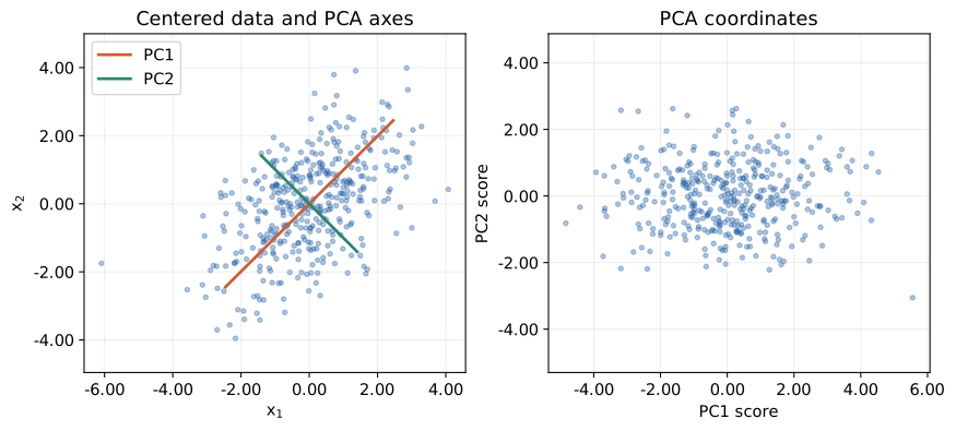
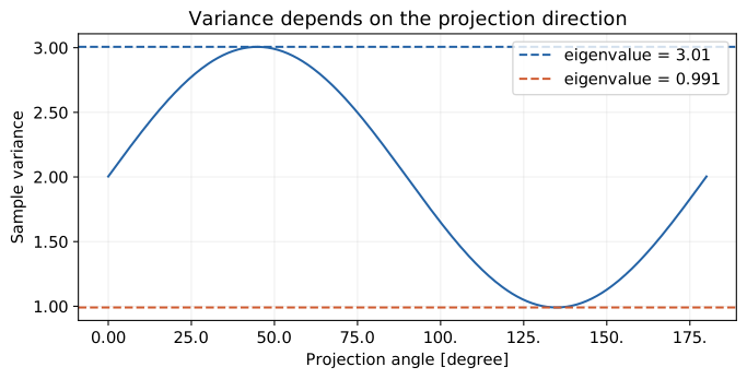
The direction with the greatest spread in the scatter plot matches the angle that maximizes the projected variance.
3. Vibration analysis: normal modes
Connect two masses to walls with three springs. Use unit spring constants and masses of one and two, with consistent units, no damping, and no external force.
$$ \ddot{x}_1=-x_1+(x_2-x_1),\quad 2\ddot{x}_2=-(x_2-x_1)-x_2, $$ $$ \mathbf{M}\ddot{\mathbf{x}}+\mathbf{K}\mathbf{x}=\mathbf{0},\quad \mathbf{M}=\begin{pmatrix}1&0\\0&2\end{pmatrix},\quad \mathbf{K}=\begin{pmatrix}2&-1\\-1&2\end{pmatrix}. $$
Substitute $\mathbf{x}(t)=\mathbf{v}\cos(\omega t)$. Since $\ddot{\mathbf{x}}=-\omega^2\mathbf{v}\cos(\omega t)$, we obtain
$$\boxed{\mathbf{K}\mathbf{v}=\omega^2\mathbf{M}\mathbf{v}}$$
The eigenvalues are squared angular frequencies. Setting $\lambda=\omega^2$ gives
$$ \det(\mathbf{K}-\lambda\mathbf{M}) =(2-\lambda)(2-2\lambda)-1 =2\lambda^2-6\lambda+3=0,\quad \lambda=\frac{6\pm\sqrt{36-24}}4=\frac{3\pm\sqrt3}2. $$
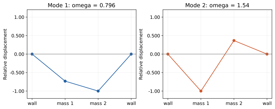
The first row gives $v_2=(2-\lambda)v_1$. Normalize so that $\mathbf{V}^{T}\mathbf{M}\mathbf{V}=\mathbf{I}$, substitute $\mathbf{x}=\mathbf{V}\mathbf{q}$, and multiply from the left by $\mathbf{V}^{T}$ to obtain $\ddot{\mathbf{q}}+\mathbf{D}\mathbf{q}=\mathbf{0}$. Each component then oscillates independently. MIT lecture on vibrations
M = np.diag([1, 2])
K = np.array([[2, -1], [-1, 2]])

# Solve the generalized eigenvalue problem directly. Eigenvector columns are normalized using the mass matrix.
omega2, modes = eigh(K, M)
omega = np.sqrt(omega2)
pprint({"omega squared": omega2, "angular frequency": omega,
        "mass-normalized modes": modes})
display(Math(r"\omega_1=" + f"{omega[0]:#.3g}"
             + r",\quad\omega_2=" + f"{omega[1]:#.3g}"))

fig, axes = plt.subplots(1, 2, figsize=(9, 3.50), layout="constrained")
for j, ax in enumerate(axes):
    shape = modes[:, j] / np.max(np.abs(modes[:, j]))
    ax.plot([0, 1, 2, 3], [0, *shape, 0], "o-", color=colors[j])
    ax.axhline(0, color="0.500", lw=1)
    ax.set(xticks=[0, 1, 2, 3], xticklabels=["wall", "mass 1", "mass 2", "wall"],
           ylim=(-1.20, 1.20), ylabel="Relative displacement",
           title=f"Mode {j + 1}: omega = {omega[j]:#.3g}")
save_figure(fig, "04_vibration_modes.svg")

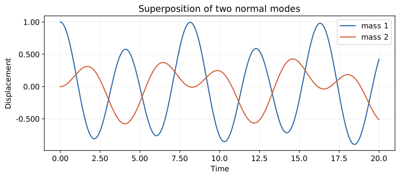
# Decompose initial displacement (1, 0) and zero initial velocity into modes and evolve them in time.
t_vibration = np.linspace(0, 20, 600)
x_initial = np.array([1, 0])
q_initial = modes.T @ M @ x_initial
q = q_initial[:, None] * np.cos(omega[:, None] * t_vibration)
q_dot = -omega[:, None] * q_initial[:, None] * np.sin(omega[:, None] * t_vibration)
x = modes @ q
x_dot = modes @ q_dot
fig, ax = plt.subplots(figsize=(8, 3.50), layout="constrained")
for j in range(2):
    ax.plot(t_vibration, x[j], color=colors[j], label=f"mass {j + 1}")
ax.set(xlabel="Time", ylabel="Displacement", title="Superposition of two normal modes")
ax.legend()
save_figure(fig, "05_vibration_time.svg")
{'angular frequency': array([0.796, 1.54]),
 'mass-normalized modes': array([[-0.460, -0.888],
       [-0.628, 0.325]]),
 'omega squared': array([0.634, 2.37])}
$$ \displaystyle \omega_1=0.796,\quad\omega_2=1.54 $$
4. Quantum mechanics: energy eigenstates
Let $\mathbf{c}(t)$ be the amplitude vector of a two-state system. For a time-independent Hermitian matrix $\mathbf{H}$, substitute $\mathbf{c}(t)=\mathbf{v}e^{-iEt/\hbar}$ into the Schrödinger equation.
$$ i\hbar\dot{\mathbf{c}}=\mathbf{H}\mathbf{c},\quad i\hbar\left(-\frac{iE}{\hbar}\right)\mathbf{v}e^{-iEt/\hbar} =\mathbf{H}\mathbf{v}e^{-iEt/\hbar}. $$
$$\boxed{\mathbf{H}\mathbf{v}=E\mathbf{v}}$$
The eigenvalues are energies. For $\mathbf{H}=g\begin{pmatrix}0&1\\1&0\end{pmatrix}$ and $g>0$, the equation $\det(\mathbf{H}-E\mathbf{I})=E^2-g^2=0$ gives $E_\pm=\pm g$ and $\mathbf{v}_\pm=(1,\pm1)^T/\sqrt2$.
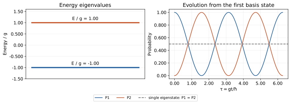
Starting from $(1,0)^T=(\mathbf{v}_++\mathbf{v}_-)/\sqrt2$ and setting $\tau=gt/\hbar$, we obtain
$$ \begin{aligned} \mathbf{c}(t)&=\frac{\mathbf{v}_+e^{-i\tau}+\mathbf{v}_-e^{i\tau}}{\sqrt2} =\frac12\begin{pmatrix}e^{-i\tau}+e^{i\tau}\\e^{-i\tau}-e^{i\tau}\end{pmatrix} =\begin{pmatrix}\cos\tau\\-i\sin\tau\end{pmatrix},\\ P_1&=|c_1|^2=\cos^2\tau,\quad P_2=|c_2|^2=\sin^2\tau. \end{aligned} $$
An energy eigenstate changes only by an overall phase, so the probabilities of the basis states remain constant. In a superposition, relative phases change and the probabilities can oscillate. MIT notes on two-state systems
# Use a dimensionless matrix, measuring energy in units of g and time in units of hbar/g.
H = np.array([[0, 1], [1, 0]])
energies, states = np.linalg.eigh(H)
tau = np.linspace(0, 2 * np.pi, 500)
c_initial = np.array([1, 0])
coefficients = states.conj().T @ c_initial
phases = np.exp(-1j * energies[:, None] * tau)
c = states @ (coefficients[:, None] * phases)
probabilities = np.abs(c) ** 2
pprint({"E / g": energies, "energy eigenstates (columns)": states})
display(Math(r"P_1+P_2=\cos^2\tau+\sin^2\tau=1"))

fig, axes = plt.subplots(1, 2, figsize=(10, 3.50), layout="constrained")
for j in range(2):
    axes[0].hlines(energies[j], 0, 1, color=colors[j], lw=3)
    axes[0].text(0.500, energies[j] + 0.120, f"E / g = {energies[j]:#.3g}", ha="center")
axes[0].set(xticks=[], ylim=(-1.50, 1.60), ylabel="Energy / g", title="Energy eigenvalues")
for j in range(2):
    axes[1].plot(tau, probabilities[j], color=colors[j], label=f"P{j + 1}")
# For a single energy eigenstate, P1 = P2 = 1/2 remains unchanged.
axes[1].axhline(1 / 2, color="0.400", ls="--", label="single eigenstate: P1 = P2")
axes[1].set(xlabel=r"$\tau = gt/\hbar$", ylabel="Probability", ylim=(-0.0500, 1.05),
           title="Evolution from the first basis state")
fig.legend(*axes[1].get_legend_handles_labels(), loc="outside lower center", ncol=3, fontsize=9)
save_figure(fig, "06_quantum_states.svg")
{'E / g': array([-1.00, 1.00]),
 'energy eigenstates (columns)': array([[-0.707, 0.707],
       [0.707, 0.707]])}
$$ \displaystyle P_1+P_2=\cos^2\tau+\sin^2\tau=1 $$
5. Graphs: differences between neighboring vertices
Let an undirected graph have weights $w_{ij}=w_{ji}\ge0$ and degrees $d_i=\sum_jw_{ij}$. From the adjacency matrix $\mathbf{W}$ and degree matrix $\mathbf{D}_g$, form $\mathbf{L}=\mathbf{D}_g-\mathbf{W}$. Then
$$ \begin{aligned} \mathbf{f}^{T}\mathbf{L}\mathbf{f} &=\sum_i d_i f_i^2-\sum_{i,j}w_{ij}f_if_j\\ &=\frac12\sum_{i,j}w_{ij}(f_i^2+f_j^2-2f_if_j)\\ &=\sum_{i<j}w_{ij}(f_i-f_j)^2\ge0. \end{aligned} $$
A constant vector has zero differences, so $\mathbf{L}\mathbf{1}=\mathbf{0}$. For a connected graph, minimize this quadratic form under $\mathbf{f}^{T}\mathbf{1}=0$ and $\mathbf{f}^{T}\mathbf{f}=1$. The stationary condition is $2\mathbf{L}\mathbf{f}-2\lambda\mathbf{f}-\mu\mathbf{1}=\mathbf{0}$. Multiplication from the left by $\mathbf{1}^{T}$ gives $-\mu n=0$, so $\mathbf{L}\mathbf{f}=\lambda\mathbf{f}$. Expanding in eigenvectors excluding the constant direction makes the quadratic form a weighted average of the remaining eigenvalues. Its minimum is the second eigenvalue, and a minimizing vector satisfies
$$\boxed{\mathbf{L}\mathbf{f}=\lambda_2\mathbf{f}}$$
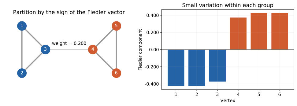
Here, $\lambda_2$ is the second-smallest eigenvalue. Splitting by the eigenvector’s sign can separate weakly connected groups, though it need not give the optimal discrete partition. Spielman’s lecture notes
# Build two complete graphs with three vertices each and join them by one weak edge.
W = np.zeros((6, 6))
for group in ([0, 1, 2], [3, 4, 5]):
    for i in group:
        for j in group:
            if i != j:
                W[i, j] = 1
W[2, 3] = W[3, 2] = 0.200
L = np.diag(W.sum(axis=1)) - W
graph_values, graph_vectors = np.linalg.eigh(L)
fiedler = graph_vectors[:, 1]
# Eigenvector signs are arbitrary; make the first component negative for consistent plots.
if fiedler[0] > 0:
    fiedler = -fiedler
# An eigenvalue that is theoretically zero can be a tiny nonzero value in floating-point arithmetic.
pprint({"Laplacian": L, "eigenvalues": graph_values,
        "Fiedler vector": fiedler})
display(Math(r"\lambda_2=" + f"{graph_values[1]:#.3g}"))

positions = np.array([[0, 1], [0, -1], [1, 0], [3, 0], [4, 1], [4, -1]])
fig, axes = plt.subplots(1, 2, figsize=(10, 3.50), layout="constrained")
for i in range(6):
    for j in range(i + 1, 6):
        if W[i, j] > 0:
            axes[0].plot(*positions[[i, j]].T, color="0.600", lw=3 * W[i, j])
node_colors = [colors[0] if value < 0 else colors[1] for value in fiedler]
axes[0].scatter(*positions.T, c=node_colors, s=500, zorder=3)
for i, point in enumerate(positions):
    axes[0].text(*point, str(i + 1), ha="center", va="center", color="white", zorder=4)
axes[0].text(2, 0.200, "weight = 0.200", ha="center")
axes[0].set(title="Partition by the sign of the Fiedler vector", aspect="equal")
axes[0].set_axis_off()
axes[0].margins(0.200)
axes[1].bar(np.arange(1, 7), fiedler, color=node_colors)
axes[1].axhline(0, color="0.400", lw=1)
axes[1].set(xlabel="Vertex", ylabel="Fiedler component", title="Small variation within each group",
            xticks=np.arange(1, 7), xticklabels=[str(i) for i in range(1, 7)])
save_figure(fig, "07_graph_partition.svg")

# Vary only the bridge weight and check how the second eigenvalue changes.
bridge_weights = np.linspace(0, 1, 101)
gaps = []
for weight in bridge_weights:
    W_trial = W.copy()
    W_trial[2, 3] = W_trial[3, 2] = weight
    L_trial = np.diag(W_trial.sum(axis=1)) - W_trial
    gaps.append(np.linalg.eigvalsh(L_trial)[1])
fig, ax = plt.subplots(figsize=(7, 3.50), layout="constrained")
ax.plot(bridge_weights, gaps, color=colors[0])
ax.scatter([W[2, 3]], [graph_values[1]], color=colors[1], label="example graph", zorder=3)
ax.set(xlabel="Bridge weight", ylabel=r"$\lambda_2$", title="The spectral gap and the connecting edge")
ax.legend()
save_figure(fig, "08_graph_gap.svg")
{'Fiedler vector': array([-0.425, -0.425, -0.373, 0.373, 0.425, 0.425]),
 'Laplacian': array([[2.00, -1.00, -1.00, 0.00, 0.00, 0.00],
       [-1.00, 2.00, -1.00, 0.00, 0.00, 0.00],
       [-1.00, -1.00, 2.20, -0.200, 0.00, 0.00],
       [0.00, 0.00, -0.200, 2.20, -1.00, -1.00],
       [0.00, 0.00, 0.00, -1.00, 2.00, -1.00],
       [0.00, 0.00, 0.00, -1.00, -1.00, 2.00]]),
 'eigenvalues': array([2.99e-16, 0.122, 3.00, 3.00, 3.00, 3.28])}
$$ \displaystyle \lambda_2=0.122 $$
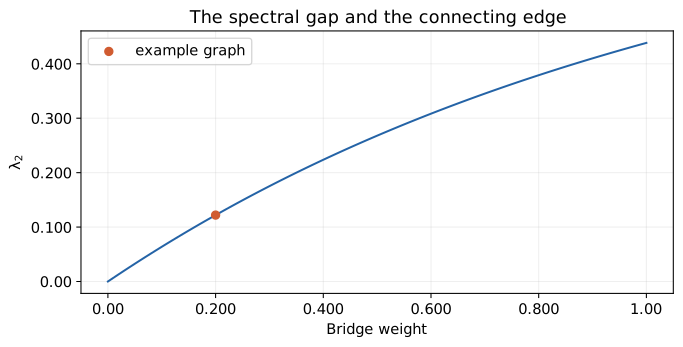
With zero bridge weight, there are two zero eigenvalues. Strengthening the bridge increases $\lambda_2$.
6. Checking the calculations
Check residuals, projected variance, conservation laws, and the quadratic form.
# Compute the same quantities from different formulas to check the derivation against the implementation.
assert np.allclose(np.var(scores, axis=0, ddof=1), pca_values)
assert np.allclose(K @ modes, (M @ modes) * omega2)
assert np.allclose(modes.T @ M @ modes, np.eye(2))
expected_omega2 = (3 + np.array([-1, 1]) * np.sqrt(3)) / 2
assert np.allclose(omega2, expected_omega2)
assert np.allclose(x[:, 0], x_initial)
energy = (np.sum(x_dot * (M @ x_dot), axis=0)
          + np.sum(x * (K @ x), axis=0)) / 2
assert np.allclose(energy, energy[0])
assert np.allclose(probabilities.sum(axis=0), 1)
assert np.allclose(probabilities[0], np.cos(tau) ** 2)
edge_energy = sum(W[i, j] * (fiedler[i] - fiedler[j]) ** 2
                  for i in range(6) for j in range(i + 1, 6))
assert np.allclose(fiedler @ L @ fiedler, edge_energy)
assert np.isclose(fiedler.sum(), 0, atol=1.00e-12)
assert np.array_equal(fiedler < 0, [True, True, True, False, False, False])

residuals = {
    "PCA": np.linalg.norm(S @ pca_vectors - pca_vectors * pca_values),
    "vibration": np.linalg.norm(K @ modes - (M @ modes) * omega2),
    "quantum": np.linalg.norm(H @ states - states * energies),
    "graph": np.linalg.norm(L @ graph_vectors - graph_vectors * graph_values),
}
assert max(residuals.values()) < 1.00e-10
# Round floating-point numbers in the dictionary only for display.
pprint({name: f"{float(value):#.3g}" for name, value in residuals.items()})
print("Checked the eigenvalue equations, conservation laws, and agreement with analytic solutions.")
{'PCA': '1.57e-16',
 'graph': '2.14e-15',
 'quantum': '0.00',
 'vibration': '4.61e-16'}
Checked the eigenvalue equations, conservation laws, and agreement with analytic solutions.
Conclusion
We examined why PCA, vibration analysis, quantum mechanics, and graphs lead to eigenvalue problems through their optimization and time-evolution equations.
The eigenvalues represent variance, squared angular frequency, energy, and variation on a graph, respectively. All use a suitable basis to separate components. Orthogonal modes were available because we used symmetric or Hermitian matrices and a positive definite mass matrix. This property does not extend directly to arbitrary matrices.