Why does the Poisson equation appear in semiconductors, heat, fluids, and gravity? (Rewritten from an earlier blog post)
Environment
Python 3.14.6, NumPy 2.5.4, SciPy 1.18.1, Matplotlib 3.11.2 (Jupyter Notebook).
This article is a rewrite of a post from around 2013–2016, with calculations performed in the environment described above.
Overview
We use gradients and divergence to see why the Poisson equation appears in different fields. We consider electric potential in semiconductors, steady temperature, pressure in incompressible fluids, and Newtonian gravity, then implement one-dimensional finite differences and a two-dimensional pressure correction in Python.
Setup
Run the code in Jupyter Notebook from top to bottom. Round numbers to three significant digits only when displaying them.
from pathlib import Path
from pprint import pprint
import platform

import numpy as np
import scipy
from scipy.sparse import diags
from scipy.sparse.linalg import spsolve
import matplotlib
import matplotlib.pyplot as plt
from matplotlib.ticker import FuncFormatter, NullFormatter
from matplotlib_inline.backend_inline import set_matplotlib_formats
from IPython.display import Latex, display

%matplotlib inline
# Save as SVG and also embed PNG output for display in untrusted notebooks.
set_matplotlib_formats('svg', 'png')

print(f'Python: {platform.python_version()}')
for module in (np, scipy, matplotlib):
    print(f'{module.__name__}: {module.__version__}')

# Save beside the notebook; also support execution from the repository root.
relative_dir = Path('rec/Interdisciplinarity/103')
notebook_dir = relative_dir if relative_dir.is_dir() else Path.cwd()
image_dir = notebook_dir / '103_nb_files'
image_dir.mkdir(exist_ok=True)


def sig3(value):
    """Display three significant digits, keeping trailing zeros."""
    return '0' if value == 0 else f'{float(value):#.3g}'


np.set_printoptions(formatter={'float_kind': sig3})
plt.rcParams.update({
    'font.family': 'DejaVu Sans',
    'font.size': 10,
    'axes.spines.top': False,
    'axes.spines.right': False,
    'lines.linewidth': 1.60,
    'svg.fonttype': 'none',
})


def show_equation(source):
    # Specify key formulas with \(...\) and convert them to $$...$$ for LaTeX display.
    assert source.startswith(r'\(') and source.endswith(r'\)')
    display(Latex('$$' + source[2:-2] + '$$'))


def save_figure(fig, filename):
    """Use three significant digits for ticks, save as SVG, and display in the notebook."""
    for ax in fig.axes:
        ax.xaxis.set_major_formatter(FuncFormatter(lambda value, _: sig3(value)))
        ax.yaxis.set_major_formatter(FuncFormatter(lambda value, _: sig3(value)))
        ax.xaxis.set_minor_formatter(NullFormatter())
        ax.yaxis.set_minor_formatter(NullFormatter())
    fig.savefig(image_dir / filename, format='svg', bbox_inches='tight')
    plt.show()
    plt.close(fig)
Python: 3.14.6
numpy: 2.5.4
scipy: 1.18.1
matplotlib: 3.11.2
1. Combining the gradient and divergence
The gradient of a scalar field $u$ describes the direction and rate of change. For a flux $\mathbf{J}=-a\nabla u$, the balance with a source $s$ over a region $V$ with outward unit normal $\mathbf{n}$ is
$$ \int_{\partial V}\mathbf{J}\cdot\mathbf{n}\,dS =\int_Vs\,dV =\int_V\nabla\cdot\mathbf{J}\,dV. $$
Since this holds for any $V$, we have $\nabla\cdot\mathbf{J}=s$. Substitution gives
$$ -\nabla\cdot(a\nabla u)=s, \qquad a=\text{constant}>0 \quad\Rightarrow\quad \nabla^2u=-\frac{s}{a}=f. $$
Here, $\nabla^2u=\partial_x^2u+\partial_y^2u+\partial_z^2u$. If $f=0$, this becomes Laplace’s equation. If $a$ varies with position, the term $\nabla a\cdot\nabla u$ also remains, so the equation is no longer a constant-coefficient Poisson equation.
show_equation(r'\(\boxed{\nabla^2u=f}\qquad\mathbf{J}=-a\nabla u\)')
$$\boxed{\nabla^2u=f}\qquad\mathbf{J}=-a\nabla u$$
2. Semiconductors: from charge to potential
In the electrostatic approximation, the electric displacement $\mathbf{D}$, electric field $\mathbf{E}$, and potential $\phi$ satisfy
$$ \begin{aligned} \nabla\cdot\mathbf{D}&=\rho_e, &\mathbf{D}&=\varepsilon\mathbf{E}, &\mathbf{E}&=-\nabla\phi,\\ -\nabla\cdot(\varepsilon\nabla\phi)&=\rho_e &\Rightarrow\quad\nabla^2\phi&=-\rho_e/\varepsilon \quad(\varepsilon=\text{constant}). \end{aligned} $$
The charge density is $\rho_e=e(p_h-n+N_D^+-N_A^-)$. Here, $e>0$ is the elementary charge, $p_h,n$ are the hole and electron densities, and $N_D^+,N_A^-$ are the ionized donor and acceptor densities. In practice, carrier densities also depend on the potential, so this equation is solved together with transport equations and other relations. Dhar, Semiconductor Device Equations
3. Heat: a temperature field with no further heat storage
Use volumetric heat capacity $C$, heat-generation density $Q$, and thermal conductivity $\kappa$. A heat balance without advection, combined with Fourier’s law, gives
$$ \begin{aligned} C\partial_tT+\nabla\cdot\mathbf{q}&=Q, &\mathbf{q}&=-\kappa\nabla T,\\ C\partial_tT-\nabla\cdot(\kappa\nabla T)&=Q,\\ \partial_tT=0,\quad\kappa=\text{constant} &\Rightarrow-\kappa\nabla^2T=Q \Rightarrow\nabla^2T=-Q/\kappa. \end{aligned} $$
At steady state, heat generation balances heat loss through the boundary. If the temperature still changes with time, the heat equation must be solved. MIT 18.336, Lecture 10
4. Fluids: using pressure to enforce incompressibility
For an incompressible fluid with constant density $\rho_f$, $\nabla\cdot\mathbf{v}=0$. Compute a predicted velocity $\mathbf{v}^*$ using all terms except pressure, then correct it over a time step $\Delta t$:
$$ \begin{aligned} \mathbf{v}^{n+1}&=\mathbf{v}^*-\frac{\Delta t}{\rho_f}\nabla p,\\ 0=\nabla\cdot\mathbf{v}^{n+1} &=\nabla\cdot\mathbf{v}^*-\frac{\Delta t}{\rho_f}\nabla^2p,\\ \nabla^2p&=\frac{\rho_f}{\Delta t}\nabla\cdot\mathbf{v}^*. \end{aligned} $$
This is the pressure equation in a projection method. It is solved at each time step to remove velocity divergence, not only at steady state. The discrete divergence, gradient, and Poisson operators must also be consistent with one another. Domino, 2006
5. Gravity: a difference in sign
In Newtonian gravity, mass density $\rho_m$, gravitational acceleration $\mathbf{g}$, and potential $\Phi$ satisfy
$$ \nabla\cdot\mathbf{g}=-4\pi G\rho_m, \qquad\mathbf{g}=-\nabla\Phi \quad\Rightarrow\quad -\nabla^2\Phi=-4\pi G\rho_m \quad\Rightarrow\quad \nabla^2\Phi=4\pi G\rho_m. $$
The field points toward positive mass, so its sign is opposite to that for positive electric charge. This is not the equation of general relativity itself. Tong, The Poisson and Laplace Equations
6. Using the same finite-difference matrix
Divide the interval $0\le x\le1$ into $N$ equal parts and set $h=1/N$. Adding Taylor expansions gives
$$ \begin{aligned} u(x_i\pm h)&=u_i\pm hu^{\prime}_i+\frac{h^2}{2}u^{\prime\prime}_i \pm\frac{h^3}{6}u^{(3)}_i+O(h^4),\\ u_{i-1}-2u_i+u_{i+1}&=h^2u^{\prime\prime}_i+O(h^4),\\ -u_{i-1}+2u_i-u_{i+1}&\approx-h^2f_i. \end{aligned} $$
For interior points, the matrix $\mathbf{A}$ has diagonal entries $2$ and neighboring entries $-1$. Add the boundary values $u(0)=a,u(1)=b$ to the first and last entries of the right-hand side. Then solve $\mathbf{A}\mathbf{u}=\mathbf{b}$.
def solve_poisson_1d(source, intervals=100, left=0, right=0):
    """Solve u'' = source(x) with Dirichlet conditions at both endpoints."""
    x = np.linspace(0, 1, intervals + 1)
    h = 1 / intervals
    size = intervals - 1
    matrix = diags(
        [-np.ones(size - 1), 2 * np.ones(size), -np.ones(size - 1)],
        offsets=[-1, 0, 1],
        format='csc',
    )
    rhs = -h**2 * np.asarray(source(x[1:-1]), dtype=float)
    rhs[0] += left
    rhs[-1] += right
    u = np.empty_like(x)
    u[0], u[-1] = left, right
    u[1:-1] = spsolve(matrix, rhs)
    return x, u


# Matrix for three interior points. Display the formula with display.
show_equation(
    r'\(\underbrace{\begin{bmatrix}2&-1&0\\-1&2&-1\\0&-1&2\end{bmatrix}}_{\mathbf{A}}'
    r'\underbrace{\begin{bmatrix}u_1\\u_2\\u_3\end{bmatrix}}_{\mathbf{u}}'
    r'=\underbrace{\begin{bmatrix}-h^2f_1+a\\-h^2f_2\\-h^2f_3+b\end{bmatrix}}_{\mathbf{b}}\)'
)
$$\underbrace{\begin{bmatrix}2&-1&0\\-1&2&-1\\0&-1&2\end{bmatrix}}_{\mathbf{A}}\underbrace{\begin{bmatrix}u_1\\u_2\\u_3\end{bmatrix}}_{\mathbf{u}}=\underbrace{\begin{bmatrix}-h^2f_1+a\\-h^2f_2\\-h^2f_3+b\end{bmatrix}}_{\mathbf{b}}$$
Comparing electric potential, temperature, and gravity
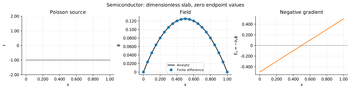
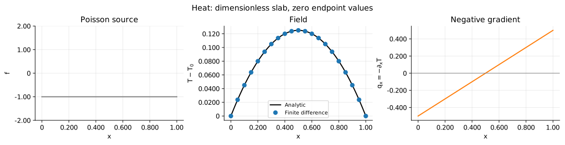
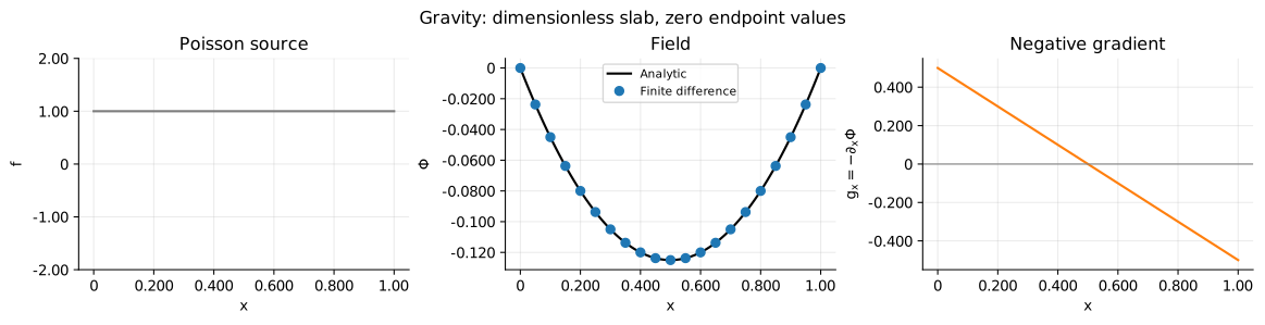
The following examples are dimensionless slab models. For the semiconductor, assume a fixed uniform positive charge; for heat, uniform heat generation; for gravity, mass that is uniform within each plane. Set the coefficients and source magnitudes to $1$ and impose $u=0$ at both ends. Temperature is measured relative to a reference. The gravitational reference is set at the slab endpoints, not at infinity as for an isolated body.
For a constant right-hand side $f=c$, integration and the boundary conditions give
$$ \begin{aligned} u^{\prime\prime}=c&\Rightarrow u^{\prime}=cx+C_1 \Rightarrow u=\frac{c}{2}x^2+C_1x+C_2,\\ u(0)=a&\Rightarrow C_2=a,\\ u(1)=b&\Rightarrow C_1=b-a-\frac{c}{2},\\ u(x)&=a+(b-a)x+\frac{c}{2}x(x-1). \end{aligned} $$
Electric potential and temperature use $c=-1$, while gravity uses $c=1$. Plot each solution alongside its negative gradient. The electric field and heat flux point outward from the center, while gravity points inward, showing the effect of the source sign.
cases = [
    ('Semiconductor', -1, r'$\phi$', r'$E_x=-\partial_x\phi$', '01_semiconductor.svg'),
    ('Heat', -1, r'$T-T_0$', r'$q_x=-\partial_xT$', '02_heat.svg'),
    ('Gravity', 1, r'$\Phi$', r'$g_x=-\partial_x\Phi$', '03_gravity.svg'),
]
checks = {}

for title, c, field_label, flux_label, filename in cases:
    x, u = solve_poisson_1d(lambda z: np.full_like(z, c))
    exact = c * x * (x - 1) / 2
    flux = -np.gradient(u, x, edge_order=2)
    exact_flux = -c * (x - 1 / 2)
    residual = np.diff(u, n=2) / (x[1] - x[0])**2 - c
    checks[title] = {
        'max_solution_error': sig3(np.max(np.abs(u - exact))),
        'max_equation_residual': sig3(np.max(np.abs(residual))),
    }
    np.testing.assert_allclose(u, exact, atol=1.00e-12)
    np.testing.assert_allclose(flux, exact_flux, atol=1.00e-12)

    fig, axes = plt.subplots(1, 3, figsize=(12, 3), layout='constrained')
    fig.suptitle(f'{title}: dimensionless slab, zero endpoint values')
    axes[0].plot(x, np.full_like(x, c), color='tab:gray')
    axes[0].set(ylabel='$f$', title='Poisson source')
    axes[0].set_ylim(-2, 2)
    axes[1].plot(x, exact, color='black', label='Analytic')
    axes[1].plot(x[::5], u[::5], 'o', color='tab:blue', label='Finite difference')
    axes[1].set(ylabel=field_label, title='Field')
    axes[1].legend(fontsize=8)
    axes[2].plot(x, flux, color='tab:orange')
    axes[2].axhline(0, color='gray', linewidth=0.800)
    axes[2].set(ylabel=flux_label, title='Negative gradient')
    for ax in axes:
        ax.set_xlabel('$x$')
        ax.grid(alpha=0.250)
    save_figure(fig, filename)

pprint(checks, sort_dicts=False)
{'Semiconductor': {'max_solution_error': '1.05e-15',
                   'max_equation_residual': '4.45e-13'},
 'Heat': {'max_solution_error': '1.05e-15',
          'max_equation_residual': '4.45e-13'},
 'Gravity': {'max_solution_error': '1.05e-15',
             'max_equation_residual': '4.45e-13'}}
Boundary conditions and errors
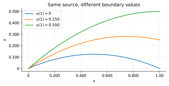
Changing boundary values changes the solution even with the same $f$. Dirichlet conditions specify values, while Neumann conditions specify normal derivatives. With Neumann conditions on the entire boundary, $\int_V f\,dV=\int_{\partial V}\partial_nu\,dS$ is required, and the additive constant in the solution must also be fixed.
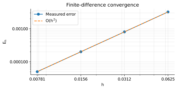
Finite differences are exact for the quadratic functions above, so use $u=\sin(\pi x)$ and $f=-\pi^2\sin(\pi x)$ to check convergence. Verify that halving the grid spacing reduces the maximum error $E_h$ to about $1/4$ of its previous value.
# Change only the right endpoint value, keeping the source and left endpoint value fixed.
fig, ax = plt.subplots(figsize=(6, 3), layout='constrained')
for right in (0, 1 / 4, 1 / 2):
    x, u = solve_poisson_1d(lambda z: -np.ones_like(z), right=right)
    exact = right * x + x * (1 - x) / 2
    np.testing.assert_allclose(u, exact, atol=1.00e-12)
    ax.plot(x, u, label=f'$u(1)={sig3(right)}$')
ax.set(xlabel='$x$', ylabel='$u$', title='Same source, different boundary values')
ax.legend()
ax.grid(alpha=0.250)
save_figure(fig, '04_boundary_conditions.svg')

# Check second-order accuracy using a nonquadratic analytic solution.
counts = np.array([16, 32, 64, 128])
errors = []
for intervals in counts:
    x, u = solve_poisson_1d(
        lambda z: -np.pi**2 * np.sin(np.pi * z), intervals=int(intervals)
    )
    errors.append(np.max(np.abs(u - np.sin(np.pi * x))))
errors = np.asarray(errors)
orders = np.log2(errors[:-1] / errors[1:])
pprint({
    'intervals': counts.tolist(),
    'max_errors': [sig3(value) for value in errors],
    'observed_orders': [sig3(value) for value in orders],
}, sort_dicts=False)
assert np.all(np.abs(orders - 2) < 0.0100)

fig, ax = plt.subplots(figsize=(6, 3), layout='constrained')
h_values = 1 / counts
ax.loglog(h_values, errors, 'o-', label='Measured error')
ax.loglog(h_values, errors[0] * (h_values / h_values[0])**2, '--', label='$O(h^2)$')
ax.set(xlabel='$h$', ylabel='$E_h$', title='Finite-difference convergence')
ax.set_xticks(h_values)
ax.legend()
ax.grid(which='both', alpha=0.250)
save_figure(fig, '05_convergence.svg')
{'intervals': [16, 32, 64, 128],
 'max_errors': ['0.00322', '0.000804', '0.000201', '5.02e-05'],
 'observed_orders': ['2.00', '2.00', '2.00']}
7. A two-dimensional pressure correction
On the periodic domain $[0,2\pi)^2$, set $\psi=\Delta t\,p/\rho_f$. The equation to solve is $\nabla^2\psi=f=\nabla\cdot\mathbf{v}^*$. In Fourier space,
$$ \nabla^2e^{i\mathbf{k}\cdot\mathbf{x}} =-|\mathbf{k}|^2e^{i\mathbf{k}\cdot\mathbf{x}} \Rightarrow-|\mathbf{k}|^2\widehat\psi=\widehat f \Rightarrow\widehat\psi=-\widehat f/|\mathbf{k}|^2. $$
For periodic boundaries, the mean of $f$ must be $0$ for a solution to exist. Avoid division at zero wave number and fix the mean by setting $\widehat\psi(\mathbf{0})=0$. Choose the example
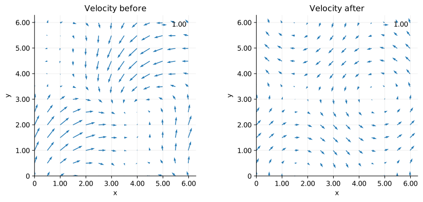
$$ \mathbf{v}^*=\begin{bmatrix}\sin x+\sin y\\\cos x+\sin y\end{bmatrix} \Rightarrow f=\cos x+\cos y \Rightarrow\psi=-\cos x-\cos y \Rightarrow\mathbf{v}=\mathbf{v}^*-\nabla\psi =\begin{bmatrix}\sin y\\\cos x\end{bmatrix} $$
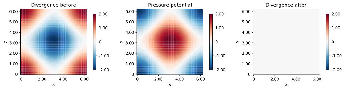
The corrected velocity has divergence exactly $0$ analytically. The code below performs one projection step, not the full time evolution of a fluid.
# Use an odd number of periodic grid points to avoid special handling of the Nyquist wave number.
size = 63
length = 2 * np.pi
grid = np.arange(size) * length / size
X, Y = np.meshgrid(grid, grid, indexing='xy')
wave = 2 * np.pi * np.fft.fftfreq(size, d=length / size)
KX, KY = np.meshgrid(wave, wave, indexing='xy')
wave_squared = KX**2 + KY**2

vx_star = np.sin(X) + np.sin(Y)
vy_star = np.cos(X) + np.sin(Y)
vx_hat = np.fft.fft2(vx_star)
vy_hat = np.fft.fft2(vy_star)

# Use the same Fourier differentiation for divergence, the Poisson equation, and the gradient.
source_hat = 1j * (KX * vx_hat + KY * vy_hat)
source = np.fft.ifft2(source_hat).real
assert abs(np.mean(source)) < 1.00e-12
psi_hat = np.zeros_like(source_hat)
nonzero = wave_squared > 0
psi_hat[nonzero] = -source_hat[nonzero] / wave_squared[nonzero]
psi = np.fft.ifft2(psi_hat).real
vx = vx_star - np.fft.ifft2(1j * KX * psi_hat).real
vy = vy_star - np.fft.ifft2(1j * KY * psi_hat).real
div_after = np.fft.ifft2(
    1j * (KX * np.fft.fft2(vx) + KY * np.fft.fft2(vy))
).real

psi_exact = -np.cos(X) - np.cos(Y)
np.testing.assert_allclose(psi, psi_exact, atol=1.00e-12)
np.testing.assert_allclose(vx, np.sin(Y), atol=1.00e-12)
np.testing.assert_allclose(vy, np.cos(X), atol=1.00e-12)
assert np.max(np.abs(div_after)) < 1.00e-12
pprint({
    'max_divergence_before': sig3(np.max(np.abs(source))),
    'max_divergence_after': sig3(np.max(np.abs(div_after))),
    'max_potential_error': sig3(np.max(np.abs(psi - psi_exact))),
}, sort_dicts=False)
show_equation(r'\(\nabla\cdot\mathbf{v}=\nabla\cdot\mathbf{v}^*-\nabla^2\psi=0\)')
{'max_divergence_before': '2.00',
 'max_divergence_after': '1.80e-14',
 'max_potential_error': '1.33e-15'}
$$\nabla\cdot\mathbf{v}=\nabla\cdot\mathbf{v}^*-\nabla^2\psi=0$$
# Use the same color range before and after correction to compare divergence reduction.
fig, axes = plt.subplots(1, 3, figsize=(12, 3), layout='constrained')
fields = [source, psi, div_after]
titles = ['Divergence before', 'Pressure potential', 'Divergence after']
for ax, field, title in zip(axes, fields, titles):
    mesh = ax.pcolormesh(
        X, Y, field, cmap='RdBu_r', vmin=-2, vmax=2, shading='nearest'
    )
    ax.set(title=title, xlabel='$x$', ylabel='$y$', aspect='equal')
    fig.colorbar(mesh, ax=ax, ticks=[-2, -1, 0, 1, 2], shrink=0.850)
save_figure(fig, '06_pressure_projection.svg')

# Also use the same arrow scale to show the remaining rotational component.
fig, axes = plt.subplots(1, 2, figsize=(9, 4), layout='constrained')
sample = (slice(None, None, 5), slice(None, None, 5))
for ax, ux, uy, title in zip(
    axes, [vx_star, vx], [vy_star, vy], ['Velocity before', 'Velocity after']
):
    arrows = ax.quiver(
        X[sample], Y[sample], ux[sample], uy[sample],
        angles='xy', scale_units='xy', scale=5, color='tab:blue',
    )
    ax.quiverkey(arrows, 0.820, 0.940, 1, '1.00', coordinates='axes', labelpos='E')
    ax.set(title=title, xlabel='$x$', ylabel='$y$', aspect='equal')
    ax.set_xlim(0, length)
    ax.set_ylim(0, length)
    ax.grid(alpha=0.200)
save_figure(fig, '07_velocity_projection.svg')

print('SVG saved to: 103_nb_files (7 files)')
SVG saved to: 103_nb_files (7 files)
Conclusion
We saw how the Poisson equation arises from combining a gradient and divergence, or from enforcing incompressibility.
The meanings of the unknown field and source differ by field, but the same numerical methods can be used. Meaningful comparisons require consistent signs, assumptions about uniform coefficients, and boundary conditions. We checked second-order accuracy in one dimension and the reduction of divergence after pressure correction in two dimensions.