Why is the exponential family important in statistics and machine learning? (Rewritten from an earlier blog post)
Environment
Python 3.14.6, NumPy 2.5.4, SciPy 1.18.1, SymPy 1.14.0, Matplotlib 3.11.2 (Jupyter Notebook).
This article is a rewrite of a post from around 2013–2016, with calculations performed in the environment described above.
Overview
The exponential family represents distributions such as Bernoulli, Poisson, and normal distributions in a common form. It is different from the single distribution called the exponential distribution. We use formulas and Python to examine means and variances, sufficient statistics, maximum likelihood, Bayesian updates, and regression models.
Setup
Run the code in Jupyter Notebook from top to bottom. Round numbers to three significant digits only when displaying them.
import sys
from base64 import b64encode
from io import BytesIO
from pathlib import Path
from pprint import pprint
from importlib.metadata import version

import numpy as np
import sympy as sp
import matplotlib.pyplot as plt
from matplotlib.ticker import FuncFormatter, MaxNLocator
from scipy import stats
from scipy.optimize import minimize
from scipy.special import expit, gammaln
from IPython.display import Math, display

print(f"Python: {sys.version.split()[0]}")
pprint({name: version(name) for name in ("numpy", "scipy", "sympy", "matplotlib")})

# Support execution from either the notebook folder or the repository root.
relative_dir = Path("rec/Interdisciplinarity/104")
notebook_dir = relative_dir if relative_dir.is_dir() else Path.cwd()
image_dir = notebook_dir / "104_nb_files"
image_dir.mkdir(exist_ok=True)


def sig3(value):
    """Display three significant digits while retaining trailing zeros."""
    return "0" if value == 0 else format(float(value), "#.3g").removesuffix(".")


np.set_printoptions(formatter={"float_kind": sig3})
plt.rcParams.update({"font.size": 11, "axes.spines.top": False,
                     "axes.spines.right": False, "svg.hashsalt": "104"})


def save_svg(fig, filename, integer_x=False):
    """Format tick labels, save as SVG, and display the figure in the output area."""
    for ax in fig.axes:
        ax.xaxis.set_major_formatter(FuncFormatter(
            lambda x, pos: f"{x:.0f}" if integer_x else sig3(x)))
        ax.yaxis.set_major_formatter(FuncFormatter(lambda y, pos: sig3(y)))
        ax.xaxis.set_major_locator(MaxNLocator(nbins=5, integer=integer_x))
        ax.yaxis.set_major_locator(MaxNLocator(nbins=5))
        ax.grid(alpha=0.200)
    path = image_dir / filename
    fig.savefig(path, format="svg", bbox_inches="tight", metadata={"Date": None})
    # Include PNG data so figures also display in untrusted notebooks.
    # Only SVG files are saved to disk.
    buffer = BytesIO()
    fig.savefig(buffer, format="png", dpi=120, bbox_inches="tight")
    plt.close(fig)
    display({"image/svg+xml": path.read_text(),
             "image/png": b64encode(buffer.getvalue()).decode("ascii")}, raw=True)
Python: 3.14.6
{'matplotlib': '3.11.2', 'numpy': '2.5.4', 'scipy': '1.18.1', 'sympy': '1.14.0'}
1. Writing distributions in a common form
First consider a single natural parameter. Here, $T(x)$ is a statistic and $h(x)$ is a factor that does not depend on the parameter.
$$p(x;\eta)=h(x)\exp\{\eta T(x)-A(\eta)\}$$
For a discrete distribution, normalization determines the log-partition function $A$.
$$ 1=e^{-A(\eta)}\sum_xh(x)e^{\eta T(x)} \quad\Rightarrow\quad A(\eta)=\log\sum_xh(x)e^{\eta T(x)}. $$
For continuous distributions, replace the sum with an integral. We assume that the support does not depend on the parameter and that, inside the natural parameter space, differentiation can be exchanged with summation or integration.
| Distribution | $\eta$ | $T(x)$ | $A(\eta)$ | $h(x)$ |
|---|---|---|---|---|
| Bernoulli | $\log\frac{q}{1-q}$ | $x$ | $\log(1+e^\eta)$ | $1$ |
| Poisson | $\log\lambda$ | $x$ | $e^\eta$ | $1/x!$ |
| Normal (variance 1) | $\mu$ | $x$ | $\eta^2/2$ | $e^{-x^2/2}/\sqrt{2\pi}$ |
Their supports are $\{0,1\}$, the nonnegative integers, and all real numbers, respectively. Assume $\lambda>0$ and $\mu\in\mathbb R$.
For example, rewriting a Bernoulli distribution with success probability $0<q<1$ gives
$$ \begin{aligned} q^x(1-q)^{1-x} &=\exp\{x\log q+(1-x)\log(1-q)\}\\ &=\exp\{x\log[q/(1-q)]+\log(1-q)\},\\ e^\eta&=q/(1-q),\quad q=e^\eta/(1+e^\eta),\\ \log(1-q)&=-\log(1+e^\eta) \end{aligned} $$
This gives the form in the table. Figure 1 shows all three distributions computed from the common form.
# Evaluate the exponential-family formulas directly and compare with SciPy distributions.
fig, axes = plt.subplots(1, 3, figsize=(12, 3), layout="constrained")

q = 0.700
x_b = np.array([0, 1])
eta_b = np.log(q / (1 - q))
prob_b = np.exp(eta_b * x_b - np.logaddexp(0, eta_b))
np.testing.assert_allclose(prob_b, stats.bernoulli.pmf(x_b, q))
axes[0].bar(x_b, prob_b, width=0.400)
axes[0].set(xlabel="x", ylabel="Probability", title=f"Bernoulli: q = {sig3(q)}")

rate = 3
x_p = np.arange(12)
eta_p = np.log(rate)
# Use log(x!) = gammaln(x + 1) to avoid computing large factorials.
prob_p = np.exp(eta_p * x_p - np.exp(eta_p) - gammaln(x_p + 1))
np.testing.assert_allclose(prob_p, stats.poisson.pmf(x_p, rate))
axes[1].bar(x_p, prob_p)
axes[1].set(xlabel="x", ylabel="Probability", title="Poisson: rate = 3")

mu = 1
x_n = np.linspace(-3, 5, 300)
density_n = np.exp(-x_n**2 / 2 + mu * x_n - mu**2 / 2) / np.sqrt(2 * np.pi)
np.testing.assert_allclose(density_n, stats.norm.pdf(x_n, loc=mu))
axes[2].plot(x_n, density_n)
axes[2].set(xlabel="x", ylabel="Density", title="Normal: mean = 1, variance = 1")
save_svg(fig, "01_distributions.svg", integer_x=True)
pprint({"Bernoulli probabilities": [sig3(v) for v in prob_b],
        "agreement with SciPy": "checked all three distributions"})
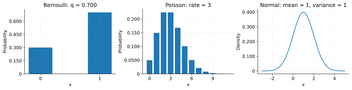
{'Bernoulli probabilities': ['0.300', '0.700'], 'agreement with SciPy': 'checked all three distributions'}
2. Derivatives give the mean and variance
Set $Z(\eta)=\sum_xh(x)e^{\eta T(x)}$, so $A=\log Z$.
$$ \begin{aligned} Z^{\prime}&=\sum_xT(x)h(x)e^{\eta T(x)},\\ A^{\prime}&=Z^{\prime}/Z=\sum_xT(x)p(x;\eta)=\mathbb E[T(X)],\\ Z^{\prime\prime}&=\sum_xT(x)^2h(x)e^{\eta T(x)},\\ A^{\prime\prime}&=\frac{Z^{\prime\prime}Z-(Z^{\prime})^2}{Z^2}\\ &=\mathbb E[T(X)^2]-\mathbb E[T(X)]^2 =\operatorname{Var}[T(X)]\geq0. \end{aligned} $$
These formulas give the mean and variance of $T(X)$. They are the mean and variance of $X$ itself when $T(x)=x$. The score for one observation is $\partial_\eta\log p=T(x)-A^{\prime}$, so the Fisher information is $I(\eta)=\mathbb E[(T(X)-A^{\prime})^2]=A^{\prime\prime}$.
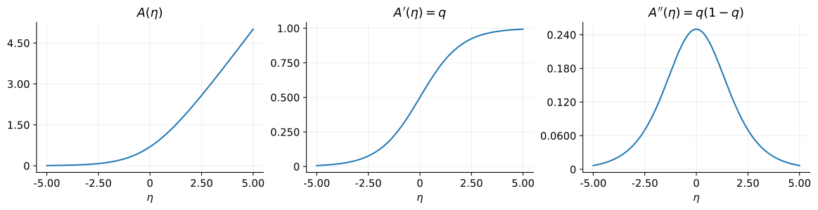
For Bernoulli, $T(X)=X$, so $A^{\prime}$ is the success probability and $A^{\prime\prime}$ the variance. Figure 2 compares the log-partition function $A$ with its first and second derivatives.
# Differentiate with SymPy and render the formulas as LaTeX output.
eta = sp.symbols("eta", real=True)
A = sp.log(1 + sp.exp(eta))
mean_expr = sp.diff(A, eta)
var_expr = sp.factor(sp.diff(A, eta, 2))
assert sp.cancel(var_expr - mean_expr * (1 - mean_expr)) == 0
display(Math(r"A'(\eta)=" + sp.latex(mean_expr)))
display(Math(r"A''(\eta)=" + sp.latex(var_expr) + r"=q(1-q)"))

eta_grid = np.linspace(-5, 5, 300)
q_grid = expit(eta_grid)
curves = [np.logaddexp(0, eta_grid), q_grid, q_grid * (1 - q_grid)]
titles = [r"$A(\eta)$", r"$A'(\eta)=q$", r"$A''(\eta)=q(1-q)$"]
fig, axes = plt.subplots(1, 3, figsize=(12, 3), layout="constrained")
for ax, values, title in zip(axes, curves, titles):
    ax.plot(eta_grid, values)
    ax.set(xlabel=r"$\eta$", title=title)
save_svg(fig, "02_log_partition.svg")
$$ \displaystyle A^{\prime}(\eta)=\frac{e^{\eta}}{e^{\eta} + 1} $$
$$ \displaystyle A^{\prime\prime}(\eta)=\frac{e^{\eta}}{\left(e^{\eta} + 1\right)^{2}}=q(1-q) $$
3. Sufficient statistics and maximum likelihood
For $n$ independent, identically distributed observations, set $S=\sum_iT(x_i)$. The likelihood factors as
$$ L(\eta)=\prod_i h(x_i)e^{\eta T(x_i)-A(\eta)} =\left(\prod_i h(x_i)\right)e^{\eta S-nA(\eta)} $$
If $n$ is known, the data enter the parameter-dependent part only through $S$. In this sense, $S$ is a sufficient statistic. This does not mean that the original data are unnecessary for checking model fit.
$$ \begin{aligned} \ell(\eta)&=\log L(\eta)=\eta S-nA(\eta)+\sum_i\log h(x_i),\\ \ell^{\prime}(\eta)&=S-nA^{\prime}(\eta),\quad \ell^{\prime\prime}(\eta)=-nA^{\prime\prime}(\eta)\leq0,\\ \ell^{\prime}(\hat\eta)=0&\quad\Rightarrow\quad A^{\prime}(\hat\eta)=S/n. \end{aligned} $$
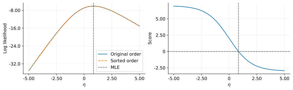
If an interior solution exists, the model expectation of $T(X)$ equals the sample mean of the observed $T(x_i)$. For seven successes in ten Bernoulli trials, $\hat q=7/10=0.700$ and $\hat\eta=\log(7/3)$. In Figure 3, differently ordered observations give overlapping log-likelihood curves.
observed = np.array([1, 0, 1, 1, 0, 1, 1, 0, 1, 1])
reordered = np.sort(observed)
n = observed.size
successes = int(observed.sum())
q_hat = successes / n
eta_hat = np.log(q_hat / (1 - q_hat))

# Compare the calculation from individual observations with the one using only the success count.
ll_full = (eta_grid[:, None] * observed - np.logaddexp(0, eta_grid[:, None])).sum(axis=1)
ll_reordered = (eta_grid[:, None] * reordered - np.logaddexp(0, eta_grid[:, None])).sum(axis=1)
ll_summary = eta_grid * successes - n * np.logaddexp(0, eta_grid)
np.testing.assert_allclose(ll_full, ll_summary)
np.testing.assert_allclose(ll_full, ll_reordered)
pprint({"n": n, "successes": successes, "estimated probability": sig3(q_hat)})
display(Math(r"\hat\eta=\log(7/3)\approx " + sig3(eta_hat)))

fig, axes = plt.subplots(1, 2, figsize=(10, 3), layout="constrained")
axes[0].plot(eta_grid, ll_full, label="Original order")
axes[0].plot(eta_grid, ll_reordered, "--", label="Sorted order")
axes[0].axvline(eta_hat, color="black", linestyle=":", label="MLE")
axes[0].set(xlabel=r"$\eta$", ylabel="Log likelihood")
axes[0].legend()
axes[1].plot(eta_grid, successes - n * expit(eta_grid))
axes[1].axhline(0, color="black", linestyle=":")
axes[1].axvline(eta_hat, color="black", linestyle=":")
axes[1].set(xlabel=r"$\eta$", ylabel="Score")
save_svg(fig, "03_sufficiency_mle.svg")
{'n': 10, 'successes': 7, 'estimated probability': '0.700'}
$$ \displaystyle \hat\eta=\log(7/3)\approx 0.847 $$
4. Updating a conjugate prior
Choose a normalizable prior $\pi(\eta)\propto e^{a\eta-bA(\eta)}$. Then
$$ \pi(\eta\mid x_1,\ldots,x_n) \propto e^{a\eta-bA(\eta)}e^{S\eta-nA(\eta)} =e^{(a+S)\eta-(b+n)A(\eta)} $$
The update stays in the same distributional form. This is conjugacy.
With a beta prior on success probability $q$, we can likewise add exponents. Assume $\alpha,\beta>0$.
$$ \begin{aligned} \pi(q\mid x_1,\ldots,x_n) &\propto q^{\alpha-1}(1-q)^{\beta-1}q^S(1-q)^{n-S}\\ &=q^{\alpha+S-1}(1-q)^{\beta+n-S-1},\\ q\mid x_1,\ldots,x_n&\sim\operatorname{Beta}(\alpha+S,\beta+n-S). \end{aligned} $$
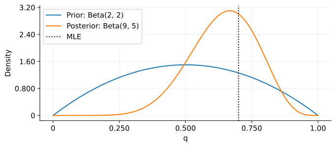
In Figure 4, $\operatorname{Beta}(2,2)$ updates to $\operatorname{Beta}(9,5)$. Additional observations only require adding success and failure counts, making this convenient for sequential updates.
alpha, beta = 2, 2
alpha_post = alpha + successes
beta_post = beta + n - successes
prob_grid = np.linspace(0, 1, 400)
posterior_mean = stats.beta.mean(alpha_post, beta_post)
pprint({"posterior parameters": [alpha_post, beta_post],
        "posterior mean": sig3(posterior_mean)})
display(Math(r"\mathbb E[q\mid x_1,\ldots,x_n]=\frac{9}{9+5}\approx "
             + sig3(posterior_mean)))

fig, ax = plt.subplots(figsize=(7, 3), layout="constrained")
ax.plot(prob_grid, stats.beta.pdf(prob_grid, alpha, beta), label="Prior: Beta(2, 2)")
ax.plot(prob_grid, stats.beta.pdf(prob_grid, alpha_post, beta_post), label="Posterior: Beta(9, 5)")
ax.axvline(q_hat, color="black", linestyle=":", label="MLE")
ax.set(xlabel="q", ylabel="Density")
ax.legend()
save_svg(fig, "04_bayes_update.svg")
{'posterior parameters': [9, 5], 'posterior mean': '0.643'}
$$ \displaystyle \mathbb E[q\mid x_1,\ldots,x_n]=\frac{9}{9+5}\approx 0.643 $$
5. The connection to logistic regression
Use a vector of explanatory variables $\mathbf{x}_i$ and coefficients $\mathbf{w}$ to form $\eta_i=\mathbf{w}^{\mathsf T}\mathbf{x}_i$. For Bernoulli,
$$q_i=A^{\prime}(\eta_i)=\frac{1}{1+e^{-\mathbf{w}^{\mathsf T}\mathbf{x}_i}}$$
The sigmoid function maps the natural parameter back to a success probability. Differentiating the negative log-likelihood $J$ for conditionally independent observations gives
$$ \begin{aligned} J(\mathbf{w})&=-\sum_i\{y_i\log q_i+(1-y_i)\log(1-q_i)\}\\ &=\sum_i\{A(\eta_i)-y_i\eta_i\},\\ \nabla J&=\sum_i\{A^{\prime}(\eta_i)-y_i\}\mathbf{x}_i =\sum_i(q_i-y_i)\mathbf{x}_i,\\ \nabla^2J&=\sum_iq_i(1-q_i)\mathbf{x}_i\mathbf{x}_i^{\mathsf T}\succeq0. \end{aligned} $$
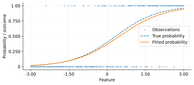
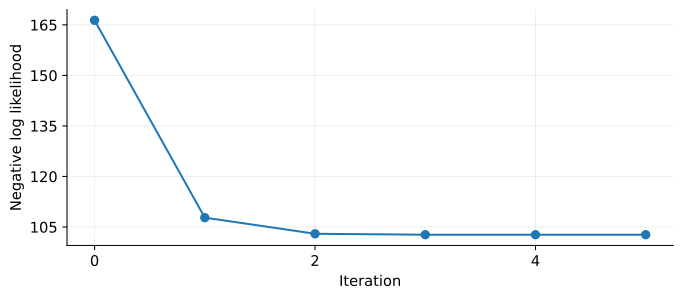
Thus, this loss is convex. The next code generates artificial data and minimizes the loss using the supplied gradient and Hessian. Figure 5 shows fitted probabilities, and Figure 6 shows the loss during optimization.
rng = np.random.default_rng(104)
feature = np.linspace(-3, 3, 240)
# The leading column of ones represents the intercept.
X = np.column_stack([np.ones(feature.size), feature])
true_w = np.array([-0.400, 1.20])
true_prob = expit(X @ true_w)
labels = rng.binomial(1, true_prob)


def loss(w):
    z = X @ w
    # Compute log(1 + exp(z)) stably.
    return float(np.sum(np.logaddexp(0, z) - labels * z))


def gradient(w):
    return X.T @ (expit(X @ w) - labels)


def hessian(w):
    p = expit(X @ w)
    return X.T @ ((p * (1 - p))[:, None] * X)


start = np.zeros(X.shape[1])
loss_history = [loss(start)]
result = minimize(loss, start, jac=gradient, hess=hessian,
                  method="trust-exact", callback=lambda w: loss_history.append(loss(w)),
                  options={"gtol": 1.00e-6})
assert result.success, result.message
assert np.linalg.norm(gradient(result.x)) < 1.00e-6
pprint({"optimization succeeded": bool(result.success),
        "estimated coefficients": [sig3(v) for v in result.x],
        "negative log-likelihood": sig3(result.fun)})

fig, ax = plt.subplots(figsize=(7, 3), layout="constrained")
ax.scatter(feature, labels, alpha=0.200, s=12, label="Observations")
ax.plot(feature, true_prob, "--", label="True probability")
ax.plot(feature, expit(X @ result.x), label="Fitted probability")
ax.set(xlabel="Feature", ylabel="Probability / outcome")
ax.legend()
save_svg(fig, "05_logistic_fit.svg")

fig, ax = plt.subplots(figsize=(7, 3), layout="constrained")
ax.plot(np.arange(len(loss_history)), loss_history, "o-")
ax.set(xlabel="Iteration", ylabel="Negative log likelihood")
save_svg(fig, "06_optimization.svg", integer_x=True)
{'estimated coefficients': ['-0.545', '1.12'], 'optimization succeeded': True, 'negative log-likelihood': '103'}
In a generalized linear model with a canonical link, the same idea applies to other distributions. The conditional mean is $e^{\eta_i}$ for Poisson and $\eta_i$ for a normal distribution with variance one.
Convexity does not guarantee a finite optimum. If a Bernoulli sample contains only successes or only failures, the maximum-likelihood natural parameter diverges. The same problem occurs with complete separation in logistic regression.
Conclusion
We used the common exponential-family form to connect moment calculations, sufficient statistics, estimation, Bayesian updating, and regression.
Many calculations can be expressed using derivatives of the log-partition function and sums of statistics. This allows shared implementations, but distributional assumptions and the existence of an estimate still need separate checks.