Why does the Rayleigh quotient appear from PCA to quantum mechanics? (Rewritten from an earlier blog post)
Environment
Python 3.14.6, NumPy 2.5.4, SciPy 1.18.1, Matplotlib 3.11.2 (Jupyter Notebook).
This article is a rewrite of a post from around 2013–2016, with calculations performed in the environment described above.
Overview
PCA maximizes projected variance, while the variational method for finding a quantum ground state minimizes expected energy. Both reduce to a Rayleigh quotient: a quadratic form divided by the squared length of a vector. We derive its connection to eigenvalues and use Python to examine two-dimensional data and a two-level system.
Setup
Run the code in Jupyter Notebook from top to bottom. Round numbers to three significant digits only when displaying them.
import platform
from pathlib import Path
from pprint import pprint

import numpy as np
import scipy
from scipy.linalg import eigh
from scipy.optimize import minimize_scalar
import matplotlib
import matplotlib.pyplot as plt
from matplotlib.ticker import FuncFormatter
from IPython.display import Math, display
from matplotlib_inline.backend_inline import set_matplotlib_formats

print(f'Python: {platform.python_version()}')
print(f'NumPy: {np.__version__} / SciPy: {scipy.__version__}')
print(f'Matplotlib: {matplotlib.__version__}')

# Support execution from either the notebook folder or the repository root.
work_dir = Path.cwd()
relative_dir = Path('rec/Interdisciplinarity/105')
notebook_dir = work_dir / relative_dir if (work_dir / relative_dir).is_dir() else work_dir
image_dir = notebook_dir / '105_nb_files'
image_dir.mkdir(exist_ok=True)

# Display decimals with three significant digits without rounding the calculations.
def sig3(value):
    return f'{float(value):#.3g}'


np.set_printoptions(formatter={'float_kind': sig3})
# Include PNG display data in the notebook so figures are visible before rerunning it.
set_matplotlib_formats('svg', 'png')
plt.rcParams.update({
    'figure.figsize': (7, 4),
    'font.size': 11,
    'axes.spines.top': False,
    'axes.spines.right': False,
    'svg.fonttype': 'none',
    'svg.hashsalt': 'rayleigh-105',
})


def save_plot(fig, filename):
    # Use the same significant-digit formatting for axes and color bars, then save as SVG.
    for ax in fig.axes:
        ax.xaxis.set_major_formatter(FuncFormatter(lambda value, _: sig3(value)))
        ax.yaxis.set_major_formatter(FuncFormatter(lambda value, _: sig3(value)))
    fig.tight_layout()
    fig.savefig(image_dir / filename, format='svg', metadata={'Date': None})
    plt.show()
    plt.close(fig)
Python: 3.14.6
NumPy: 2.5.4 / SciPy: 1.18.1
Matplotlib: 3.11.2
1. A quadratic form independent of length
For a real symmetric matrix $\mathbf{A}$ and a nonzero vector $\mathbf{x}$, define the Rayleigh quotient.
$$ R_{\mathbf{A}}(\mathbf{x})= \frac{\mathbf{x}^{T}\mathbf{A}\mathbf{x}}{\mathbf{x}^{T}\mathbf{x}}. $$
Multiplying by a real number $a\ne0$ scales the numerator and denominator by the same factor, which cancels.
$$ R_{\mathbf{A}}(a\mathbf{x}) =\frac{a^2\mathbf{x}^{T}\mathbf{A}\mathbf{x}}{a^2\mathbf{x}^{T}\mathbf{x}} =R_{\mathbf{A}}(\mathbf{x}). $$
Thus, it is enough to fix the length at one and vary only the direction.
Why eigenvalues give the bounds
Let $\mathbf{u}_i$ be orthonormal eigenvectors with eigenvalues $\lambda_i$, and expand $\mathbf{x}=\sum_i c_i\mathbf{u}_i$. Using orthogonality, $\mathbf{u}_i^T\mathbf{u}_j=\delta_{ij}$, gives
$$ \begin{aligned} \mathbf{x}^{T}\mathbf{A}\mathbf{x} &=\sum_{i,j}c_i c_j\lambda_j\mathbf{u}_i^T\mathbf{u}_j =\sum_i\lambda_i c_i^2,\\ \mathbf{x}^{T}\mathbf{x}&=\sum_{i,j}c_i c_j\delta_{ij}=\sum_i c_i^2,\\ R_{\mathbf{A}}(\mathbf{x})&=\sum_i p_i\lambda_i, \qquad p_i=\frac{c_i^2}{\sum_j c_j^2},\quad \sum_i p_i=1. \end{aligned} $$
Since $p_i\ge0$, the Rayleigh quotient is a weighted average of the eigenvalues.
$$ \lambda_{\min}\le R_{\mathbf{A}}(\mathbf{x})\le\lambda_{\max}. $$
Both bounds are attained by nonzero vectors in the corresponding eigenspaces. This is the same result as the variational characterization of eigenvalues.
We also derive the stationary condition. Set $f=\mathbf{x}^T\mathbf{A}\mathbf{x}$ and $g=\mathbf{x}^T\mathbf{x}$. Then
$$ \begin{aligned} \nabla f&=(\mathbf{A}+\mathbf{A}^T)\mathbf{x}=2\mathbf{A}\mathbf{x}, \quad \nabla g=2\mathbf{x},\\ \nabla R&=\frac{g\nabla f-f\nabla g}{g^2} =\frac{2}{g}(\mathbf{A}\mathbf{x}-R\mathbf{x}),\\ \nabla R=\mathbf{0}&\ \Longleftrightarrow\ \mathbf{A}\mathbf{x}=R\mathbf{x}. \end{aligned} $$
Stationary points are eigenvectors. Those associated with intermediate eigenvalues need not be maxima or minima.
A two-dimensional example
$$ \mathbf{A}=\begin{pmatrix}4&1\\1&2\end{pmatrix},\qquad \mathbf{x}(\theta)=\begin{pmatrix}\cos\theta\\\sin\theta\end{pmatrix}. $$
$$ \begin{aligned} R(\theta)&=4\cos^2\theta+2\sin\theta\cos\theta+2\sin^2\theta\\ &=3+\cos2\theta+\sin2\theta,\\ \det(\mathbf{A}-\lambda\mathbf{I})&=(4-\lambda)(2-\lambda)-1 =\lambda^2-6\lambda+7=0,\\ \lambda&=3\pm\sqrt{2}. \end{aligned} $$
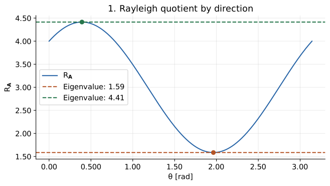
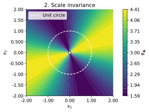
Figure 1 plots the Rayleigh quotient against direction. In Figure 2, excluding the origin, the color is constant along each ray from the origin. This shows that changing a vector’s length does not change its Rayleigh quotient.
def rayleigh(matrix, vector):
    # vdot conjugates its first argument. Assume matrix is real symmetric or Hermitian.
    norm_squared = np.vdot(vector, vector).real
    if norm_squared == 0:
        raise ValueError('The Rayleigh quotient is undefined for the zero vector.')
    return float((np.vdot(vector, matrix @ vector) / norm_squared).real)


A = np.array([[4, 1], [1, 2]], dtype=float)
eigenvalues, eigenvectors = eigh(A)  # Eigenvalues are returned in ascending order.
pprint({'A': A, 'eigenvalues': eigenvalues})
display(Math(r'\lambda_{\min}=3-\sqrt{2}\approx' + sig3(eigenvalues[0])
             + r',\qquad\lambda_{\max}=3+\sqrt{2}\approx' + sig3(eigenvalues[1])))

angles = np.linspace(0, np.pi, 501)
directions = np.column_stack((np.cos(angles), np.sin(angles)))
quotients = np.array([rayleigh(A, vector) for vector in directions])
fig, ax = plt.subplots()
ax.plot(angles, quotients, color='#2563a6', label=r'$R_{\mathbf{A}}$')
for index, color in [(0, '#b45426'), (1, '#26764b')]:
    direction = eigenvectors[:, index]
    angle = np.arctan2(direction[1], direction[0]) % np.pi
    value = eigenvalues[index]
    ax.axhline(value, color=color, linestyle='--', label=f'Eigenvalue: {sig3(value)}')
    ax.scatter(angle, value, color=color, zorder=3)
ax.set(xlabel=r'$\theta$ [rad]', ylabel=r'$R_{\mathbf{A}}$', title='1. Rayleigh quotient by direction')
ax.legend()
ax.grid(alpha=0.250)
save_plot(fig, '01_rayleigh_angle.svg')
{'A': array([[4.00, 1.00],
       [1.00, 2.00]]),
 'eigenvalues': array([1.59, 4.41])}
$$ \displaystyle \lambda_{\min}=3-\sqrt{2}\approx1.59,\qquad\lambda_{\max}=3+\sqrt{2}\approx4.41 $$
# Leave the origin undefined and display it as a hole.
grid = np.linspace(-2, 2, 241)
xx, yy = np.meshgrid(grid, grid)
norm_squared = xx**2 + yy**2
field = np.full_like(xx, np.nan)
np.divide(4 * xx**2 + 2 * xx * yy + 2 * yy**2, norm_squared,
          out=field, where=norm_squared > 0)

fig, ax = plt.subplots()
contour = ax.contourf(xx, yy, field, levels=np.linspace(*eigenvalues, 25), cmap='viridis')
circle = np.linspace(0, 2 * np.pi, 301)
ax.plot(np.cos(circle), np.sin(circle), color='white', linestyle='--', label='Unit circle')
ax.scatter(0, 0, facecolor='white', edgecolor='black', s=45, zorder=3)
ax.set(xlabel=r'$x_1$', ylabel=r'$x_2$', title='2. Scale invariance', aspect='equal')
fig.colorbar(contour, ax=ax, label=r'$R_{\mathbf{A}}$')
ax.legend(loc='upper left')
save_plot(fig, '02_rayleigh_plane.svg')
2. PCA maximizes variance
Arrange $n$ observations in rows and subtract each column mean to form $\mathbf{X}$. We do not standardize the variables here. Projection onto a unit vector $\mathbf{w}$ gives $\mathbf{y}=\mathbf{X}\mathbf{w}$, whose mean is also zero.
$$ \begin{aligned} s_y^2&=\frac{\sum_{k=1}^n y_k^2}{n-1} =\frac{\mathbf{y}^T\mathbf{y}}{n-1} =\frac{\mathbf{w}^T\mathbf{X}^T\mathbf{X}\mathbf{w}}{n-1}\\ &=\mathbf{w}^T\mathbf{C}\mathbf{w}=R_{\mathbf{C}}(\mathbf{w}), \qquad\mathbf{C}=\frac{\mathbf{X}^T\mathbf{X}}{n-1}. \end{aligned} $$
The first principal-component direction therefore corresponds to the largest eigenvalue of the covariance matrix $\mathbf{C}$. Choose later directions subject to orthogonality to the earlier ones. This is the connection between PCA variances and eigenvalues.
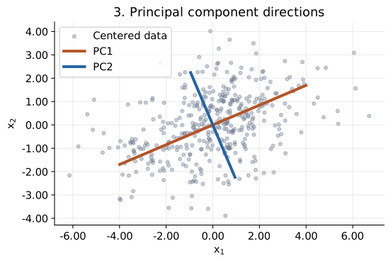
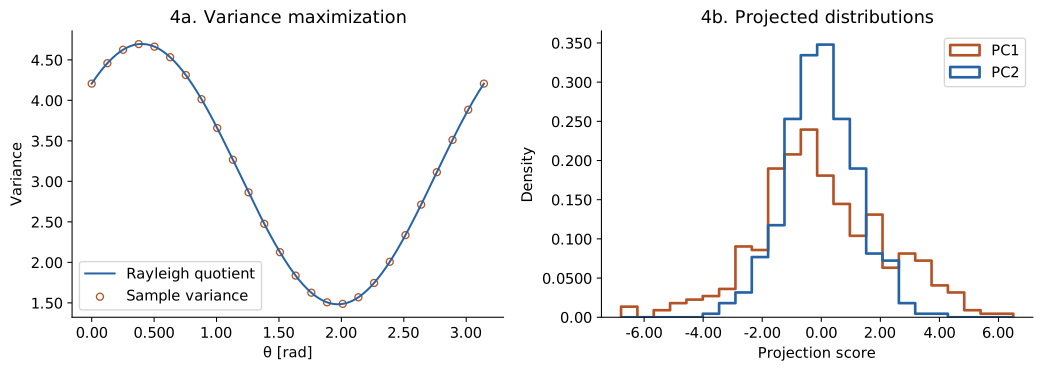
Generate random data with population covariance equal to the earlier $\mathbf{A}$. The sample covariance $\mathbf{C}$ need not equal $\mathbf{A}$. Each line in Figure 3 has half-length equal to twice the standard deviation of that principal component. Figure 4 overlays the variance computed directly from projected values with the Rayleigh quotient, and also compares the component distributions.
rng = np.random.default_rng(105)
observations = rng.multivariate_normal(mean=[0, 0], cov=A, size=400)
X = observations - observations.mean(axis=0)
C = X.T @ X / (len(X) - 1)
variances, components = eigh(C)
variances = variances[::-1]
components = components[:, ::-1]  # Order from the first principal component onward.
scores = X @ components
pprint({'sample_covariance': C, 'PC_variances': variances,
        'explained_variance_ratio': variances / variances.sum()})
display(Math(r's_{\mathrm{PC1}}^2=\lambda_{\max}(\mathbf{C})\approx'
             + sig3(variances[0])))

fig, ax = plt.subplots()
ax.scatter(X[:, 0], X[:, 1], s=14, alpha=0.350, color='#64748b', label='Centered data')
for index, color in [(0, '#b45426'), (1, '#2563a6')]:
    extent = 2 * np.sqrt(variances[index]) * components[:, index]
    ax.plot([-extent[0], extent[0]], [-extent[1], extent[1]],
            color=color, linewidth=3, label=f'PC{index + 1}')
ax.set(xlabel=r'$x_1$', ylabel=r'$x_2$', title='3. Principal component directions', aspect='equal')
ax.legend()
ax.grid(alpha=0.250)
save_plot(fig, '03_pca_directions.svg')
{'PC_variances': array([4.70, 1.48]),
 'explained_variance_ratio': array([0.760, 0.240]),
 'sample_covariance': array([[4.21, 1.15],
       [1.15, 1.97]])}
$$ \displaystyle s_{\mathrm{PC1}}^2=\lambda_{\max}(\mathbf{C})\approx4.70 $$
projected_variance = np.var(X @ directions.T, axis=0, ddof=1)
covariance_quotient = np.array([rayleigh(C, vector) for vector in directions])
fig, axes = plt.subplots(1, 2, figsize=(11, 4))
axes[0].plot(angles, covariance_quotient, label='Rayleigh quotient', color='#2563a6')
axes[0].scatter(angles[::20], projected_variance[::20], s=28,
                facecolor='none', edgecolor='#b45426', label='Sample variance')
axes[0].set(xlabel=r'$\theta$ [rad]', ylabel='Variance', title='4a. Variance maximization')
axes[0].legend()

# Use the same bins to compare the spread of each principal component.
bins = np.linspace(scores.min(), scores.max(), 25)
for index, color in [(0, '#b45426'), (1, '#2563a6')]:
    axes[1].hist(scores[:, index], bins=bins, density=True, histtype='step',
                 linewidth=2, color=color, label=f'PC{index + 1}')
axes[1].set(xlabel='Projection score', ylabel='Density', title='4b. Projected distributions')
axes[1].legend()
save_plot(fig, '04_pca_variance.svg')
3. Quantum mechanics: finding a ground state by minimizing energy
In a finite-dimensional quantum system, the Hamiltonian is a Hermitian matrix $\mathbf{H}=\mathbf{H}^{\dagger}$, where $\dagger$ denotes the conjugate transpose. The energy expectation for a state vector $\mathbf{z}\ne\mathbf{0}$ is also a Rayleigh quotient.
$$ E(\mathbf{z})=\frac{\mathbf{z}^{\dagger}\mathbf{H}\mathbf{z}} {\mathbf{z}^{\dagger}\mathbf{z}} =\frac{\sum_j E_j|c_j|^2}{\sum_j|c_j|^2}\ge E_0. $$
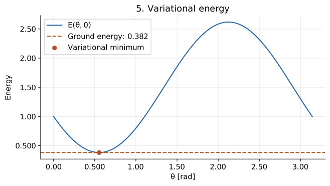
Here, $\mathbf{z}=\sum_j c_j\mathbf{v}_j$, $\mathbf{H}\mathbf{v}_j=E_j\mathbf{v}_j$, and $E_0$ is the smallest eigenvalue. Replace $c_j^2$ by $|c_j|^2$ in the real-valued derivation. Minimizing the expected energy over a restricted set of trial states gives an upper bound on the true ground-state energy. This is the variational principle.
Use a two-level model with a fixed energy unit.
$$ \begin{aligned} \mathbf{H}&=\begin{pmatrix}1&-1\\-1&2\end{pmatrix},\\ \det(\mathbf{H}-E\mathbf{I})&=(1-E)(2-E)-1=E^2-3E+1=0,\\ E_0&=\frac{3-\sqrt5}{2},\qquad E_1=\frac{3+\sqrt5}{2}. \end{aligned} $$
Write a normalized state as $\mathbf{z}=(\cos\theta,e^{i\phi}\sin\theta)^T$, and abbreviate $c=\cos\theta$ and $s=\sin\theta$. Then
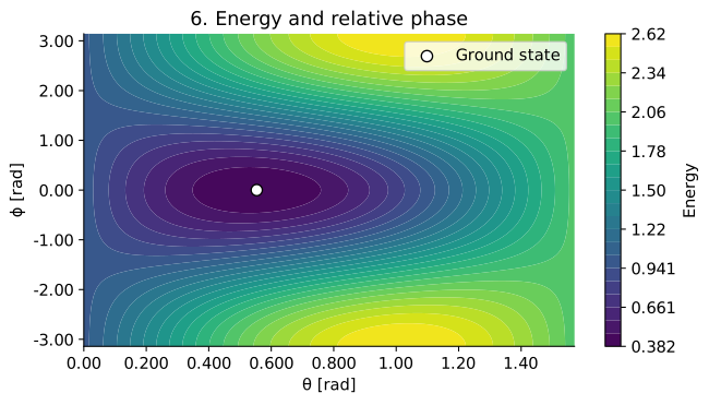
$$ \begin{aligned} E(\theta,\phi)&=c(c-e^{i\phi}s)+e^{-i\phi}s(-c+2e^{i\phi}s)\\ &=c^2+2s^2-(e^{i\phi}+e^{-i\phi})cs\\ &=\cos^2\theta+2\sin^2\theta-2\cos\theta\sin\theta\cos\phi. \end{aligned} $$
In Figure 5, fix $\phi=0$ and optimize the angle. This model has a real ground state, so the restricted calculation can recover the exact minimum. Figure 6 also varies the relative phase. Even with the same component magnitudes, changing the relative phase changes the energy expectation.
H = np.array([[1, -1], [-1, 2]], dtype=float)
energies, states = eigh(H)


def trial_state(theta, phase=0):
    return np.array([np.cos(theta), np.exp(1j * phase) * np.sin(theta)])


def trial_energy(theta, phase=0):
    return rayleigh(H, trial_state(theta, phase))


# Both components of the ground state can be chosen nonnegative in this model.
optimum = minimize_scalar(trial_energy, bounds=(0, np.pi / 2), method='bounded')
assert optimum.success
pprint({'energy_eigenvalues': energies,
        'theta_min': sig3(optimum.x), 'variational_energy': sig3(optimum.fun)})
display(Math(r'E_0=\frac{3-\sqrt5}{2}\approx' + sig3(energies[0])
             + r',\qquad E(\theta_*,0)\approx' + sig3(optimum.fun)))

energy_curve = np.array([trial_energy(theta) for theta in angles])
fig, ax = plt.subplots()
ax.plot(angles, energy_curve, color='#2563a6', label=r'$E(\theta,0)$')
ax.axhline(energies[0], color='#b45426', linestyle='--', label=f'Ground energy: {sig3(energies[0])}')
ax.scatter(optimum.x, optimum.fun, color='#b45426', zorder=3, label='Variational minimum')
ax.set(xlabel=r'$\theta$ [rad]', ylabel='Energy', title='5. Variational energy')
ax.legend()
ax.grid(alpha=0.250)
save_plot(fig, '05_quantum_energy.svg')
{'energy_eigenvalues': array([0.382, 2.62]),
 'theta_min': '0.554',
 'variational_energy': '0.382'}
$$ \displaystyle E_0=\frac{3-\sqrt5}{2}\approx0.382,\qquad E(\theta_*,0)\approx0.382 $$
theta_grid = np.linspace(0, np.pi / 2, 181)
phase_grid = np.linspace(-np.pi, np.pi, 241)
tt, pp = np.meshgrid(theta_grid, phase_grid)
energy_map = (np.cos(tt)**2 + 2 * np.sin(tt)**2
              - 2 * np.cos(tt) * np.sin(tt) * np.cos(pp))
fig, ax = plt.subplots()
contour = ax.contourf(tt, pp, energy_map, levels=np.linspace(*energies, 25), cmap='viridis')
ax.scatter(optimum.x, 0, color='white', edgecolor='black', s=60, label='Ground state')
ax.set(xlabel=r'$\theta$ [rad]', ylabel=r'$\phi$ [rad]', title='6. Energy and relative phase')
fig.colorbar(contour, ax=ax, label='Energy')
ax.legend()
save_plot(fig, '06_quantum_phase.svg')

# Check consistency between analytic formulas, eigenvalues, projected variance, and variational calculations.
np.testing.assert_allclose(eigenvalues, [3 - np.sqrt(2), 3 + np.sqrt(2)])
np.testing.assert_allclose(projected_variance, covariance_quotient)
np.testing.assert_allclose(np.var(scores, axis=0, ddof=1), variances)
np.testing.assert_allclose(optimum.fun, energies[0], atol=1.00e-10)
sample_theta, sample_phase = tt[::20, ::20], pp[::20, ::20]
direct_energy = np.array([
    trial_energy(theta, phase)
    for theta, phase in zip(sample_theta.ravel(), sample_phase.ravel())
]).reshape(sample_theta.shape)
np.testing.assert_allclose(direct_energy, energy_map[::20, ::20])
assert energy_map.min() >= energies[0] - 1.00e-12
assert energy_map.max() <= energies[1] + 1.00e-12
print('Checked agreement between analytic formulas and numerical calculations. Saved six SVG files.')
Checked agreement between analytic formulas and numerical calculations. Saved six SVG files.
Conclusion
We showed that maximizing variance in PCA and minimizing energy in quantum mechanics both reduce to eigenvalue bounds on the Rayleigh quotient.
Both compare normalized quadratic forms over directions or states. PCA seeks the largest eigenvalue of a covariance matrix, while a quantum ground-state problem seeks the smallest eigenvalue of a Hamiltonian. This shared mathematical structure explains why the same quotient appears.