Deriving OLS from maximum likelihood (Rewritten from an earlier blog post)
Environment
Python 3.14.6, NumPy 2.5.4, SciPy 1.18.1, Matplotlib 3.11.2 (Jupyter Notebook).
This article is a rewrite of a post from around 2013–2016, with calculations performed in the environment described above.
Overview
Ordinary least squares (OLS) minimizes the residual sum of squares. Assuming independent normal errors with equal variance, we derive OLS from the likelihood. We use Python and plots to examine estimates of the coefficients and error variance.
Setup
Run the code in Jupyter Notebook from top to bottom. Round numbers to three significant digits only when displaying them.
import base64
import platform
from io import BytesIO
from pathlib import Path
from pprint import pprint

import matplotlib
import matplotlib.pyplot as plt
import numpy as np
import scipy
from IPython.display import Latex, display
from matplotlib.ticker import FuncFormatter
from scipy.optimize import minimize
from scipy.stats import norm

print(f"Python: {platform.python_version()}")
print(f"NumPy: {np.__version__}, SciPy: {scipy.__version__}")
print(f"Matplotlib: {matplotlib.__version__}")


def sig3(value):
    # Keep trailing zeros to display three significant digits.
    return format(float(value), "#.3g")


np.set_printoptions(formatter={"float_kind": sig3})
plt.rcParams.update({"font.size": 11, "axes.grid": True,
                     "grid.alpha": 0.250, "svg.hashsalt": "ols-101"})
image_dir = Path("101_nb_files")
image_dir.mkdir(exist_ok=True)


def save_svg(fig, filename):
    # Apply the same formatting to axis and color-bar tick labels.
    for ax in fig.axes:
        ax.xaxis.set_major_formatter(FuncFormatter(lambda x, _: sig3(x)))
        ax.yaxis.set_major_formatter(FuncFormatter(lambda y, _: sig3(y)))
    path = image_dir / filename
    fig.savefig(path, format="svg", bbox_inches="tight", metadata={"Date": None})
    # Also create an in-memory PNG for viewers that do not allow SVG.
    png_buffer = BytesIO()
    fig.savefig(png_buffer, format="png", dpi=150, bbox_inches="tight")
    plt.close(fig)
    display({"image/svg+xml": path.read_text(encoding="utf-8"),
             "image/png": base64.b64encode(png_buffer.getvalue()).decode("ascii")},
            raw=True)
Python: 3.14.6
NumPy: 2.5.4, SciPy: 1.18.1
Matplotlib: 3.11.2
1. The linear model and error assumptions
Let $n$ be the number of observations and $p$ the number of coefficients, including the intercept. Treat the explanatory variables as fixed and write the model in matrix-vector form.
$$ \mathbf{y}=\mathbf{X}\mathbf{b}+\mathbf{u},\qquad \mathbf{y},\mathbf{u}\in\mathbb{R}^{n},\quad \mathbf{X}\in\mathbb{R}^{n\times p},\quad \mathbf{b}\in\mathbb{R}^{p}. $$
If row $i$ of $\mathbf{X}$ is $\mathbf{x}_i^{\mathsf T}$, then $y_i=\mathbf{x}_i^{\mathsf T}\mathbf{b}+u_i$. Conditional on the explanatory variables, assume the $u_i$ are independent, with $u_i\sim N(0,v)$ and $v=\sigma^2>0$. The conditional density of each observation is therefore
$$ f(y_i\mid\mathbf{x}_i,\mathbf{b},v) =\frac{1}{\sqrt{2\pi v}} \exp\left[-\frac{(y_i-\mathbf{x}_i^{\mathsf T}\mathbf{b})^2}{2v}\right] $$
In what follows, assume $n>p$ and $\operatorname{rank}(\mathbf{X})=p$. Normality is needed for this connection to maximum likelihood, but not for computing OLS itself.
2. Taking the logarithm of the likelihood
Independence makes the joint density a product. Holding the observations fixed and viewing it as a function of the unknown parameters $\mathbf{b},v$ gives the likelihood.
$$ \begin{aligned} L(\mathbf{b},v) &=\prod_{i=1}^{n}\frac{1}{\sqrt{2\pi v}} \exp\left[-\frac{(y_i-\mathbf{x}_i^{\mathsf T}\mathbf{b})^2}{2v}\right]\\ &=(2\pi v)^{-n/2}\exp\left[-\frac{1}{2v} \sum_{i=1}^{n}(y_i-\mathbf{x}_i^{\mathsf T}\mathbf{b})^2\right],\\ S(\mathbf{b})&=\sum_{i=1}^{n}(y_i-\mathbf{x}_i^{\mathsf T}\mathbf{b})^2,\\ \ell(\mathbf{b},v)=\log L(\mathbf{b},v) &=-\frac n2\log(2\pi)-\frac n2\log v-\frac{S(\mathbf{b})}{2v}. \end{aligned} $$
The logarithm is strictly increasing, so it preserves the maximum. For fixed $v>0$, the first two terms do not depend on the coefficients, and the factor $-1/(2v)$ multiplying $S$ is negative. Thus, a smaller residual sum of squares $S$ means a larger log-likelihood, and both criteria give the same optimal coefficients.
3. Differentiating to obtain OLS
Expand the residual sum of squares. The two middle terms are equal because they are scalars that are transposes of each other.
$$ \begin{aligned} S(\mathbf{b}) &=(\mathbf{y}-\mathbf{X}\mathbf{b})^{\mathsf T} (\mathbf{y}-\mathbf{X}\mathbf{b})\\ &=\mathbf{y}^{\mathsf T}\mathbf{y} -\mathbf{y}^{\mathsf T}\mathbf{X}\mathbf{b} -\mathbf{b}^{\mathsf T}\mathbf{X}^{\mathsf T}\mathbf{y} +\mathbf{b}^{\mathsf T}\mathbf{X}^{\mathsf T}\mathbf{X}\mathbf{b}\\ &=\mathbf{y}^{\mathsf T}\mathbf{y} -2\mathbf{b}^{\mathsf T}\mathbf{X}^{\mathsf T}\mathbf{y} +\mathbf{b}^{\mathsf T}\mathbf{X}^{\mathsf T}\mathbf{X}\mathbf{b}. \end{aligned} $$
Collecting the derivatives with respect to the components $b_j$ gives the gradient.
$$ \begin{aligned} \frac{\partial S}{\partial b_j} &=\sum_i2\left(y_i-\sum_kx_{ik}b_k\right)(-x_{ij}),\\ \nabla_{\mathbf{b}}S &=-2\mathbf{X}^{\mathsf T}(\mathbf{y}-\mathbf{X}\mathbf{b}),\\ \nabla_{\mathbf{b}}\ell &=-\frac{1}{2v}\nabla_{\mathbf{b}}S =\frac{1}{v}\mathbf{X}^{\mathsf T}(\mathbf{y}-\mathbf{X}\mathbf{b}). \end{aligned} $$
Setting the gradient to zero gives the normal equations.
$$ \mathbf{X}^{\mathsf T}\mathbf{y} -\mathbf{X}^{\mathsf T}\mathbf{X}\hat{\mathbf{b}}=\mathbf{0} \quad\Longrightarrow\quad \boxed{\hat{\mathbf{b}}=(\mathbf{X}^{\mathsf T}\mathbf{X})^{-1} \mathbf{X}^{\mathsf T}\mathbf{y}}. $$
The Hessian of the log-likelihood is $-\mathbf{X}^{\mathsf T}\mathbf{X}/v$. For any nonzero vector $\mathbf{a}$, $-\mathbf{a}^{\mathsf T}\mathbf{X}^{\mathsf T}\mathbf{X}\mathbf{a}/v=-\|\mathbf{X}\mathbf{a}\|^2/v<0$, so the maximum is unique for fixed $v$. If the columns are not independent, the coefficients are not unique and the inverse above does not exist.
4. Estimating the unknown variance
Assume $S_*=S(\hat{\mathbf{b}})>0$. Fix the coefficients at their estimates and differentiate with respect to the variance.
$$ \begin{aligned} \frac{\partial\ell}{\partial v} &=-\frac{n}{2v}+\frac{S_*}{2v^2} =\frac{S_*-nv}{2v^2},\\ \frac{\partial\ell}{\partial v}=0 &\Longleftrightarrow S_*-nv=0 \Longleftrightarrow\hat v_{\mathrm{ML}}=\frac{S_*}{n}. \end{aligned} $$
The derivative is positive for $v<S_*/n$ and negative for $v>S_*/n$. Since the maximizing coefficients are the same for every $v$, this pair gives the joint maximum-likelihood estimate. If $S_*=0$, the likelihood diverges as $v\to0$, so it has no finite maximum at a positive variance.
The maximum-likelihood variance estimate is biased. Under the same model, $E[S_*]=(n-p)v$, so
$$ E[\hat v_{\mathrm{ML}}]=\frac{n-p}{n}v, \qquad s^2=\frac{S_*}{n-p},\qquad E[s^2]=v. $$
Estimating the coefficients reduces the residual degrees of freedom. Whether the denominator is $n$ or $n-p$ reflects a difference in the estimation method.
# Also display the main results in LaTeX form.
display(Latex(
    r"\(\boxed{\hat{\mathbf{b}}_{\mathrm{ML}}=\hat{\mathbf{b}}_{\mathrm{OLS}}"
    r"=(\mathbf{X}^{\mathsf T}\mathbf{X})^{-1}\mathbf{X}^{\mathsf T}\mathbf{y}},"
    r"\quad\boxed{\hat\sigma^2_{\mathrm{ML}}=S_*/n}\)"
))
$$ \boxed{\hat{\mathbf{b}}_{\mathrm{ML}}=\hat{\mathbf{b}}_{\mathrm{OLS}}=(\mathbf{X}^{\mathsf T}\mathbf{X})^{-1}\mathbf{X}^{\mathsf T}\mathbf{y}},\quad\boxed{\hat\sigma^2_{\mathrm{ML}}=S_*/n} $$
5. A small worked example
Fit $y_i\approx b_0+b_1x_i$ to the four points $(x_i,y_i)=(0,1),(1,2),(2,2),(3,4)$.
$$ \mathbf{X}=\begin{bmatrix}1&0\\1&1\\1&2\\1&3\end{bmatrix},\quad \mathbf{y}=\begin{bmatrix}1\\2\\2\\4\end{bmatrix},\quad \mathbf{X}^{\mathsf T}\mathbf{X}=\begin{bmatrix}4&6\\6&14\end{bmatrix},\quad \mathbf{X}^{\mathsf T}\mathbf{y}=\begin{bmatrix}9\\18\end{bmatrix}. $$
The normal equations are $4b_0+6b_1=9$ and $6b_0+14b_1=18$. Subtracting three times the first equation from twice the second gives $10b_1=9$. Thus, $b_1=0.900$ and $b_0=(9-6\times0.900)/4=0.900$.
$$ \mathbf{r}=\begin{bmatrix}0.100\\0.200\\-0.700\\0.400\end{bmatrix},\quad S_*=0.100^2+0.200^2+(-0.700)^2+0.400^2=0.700. $$
Therefore, $\hat v_{\mathrm{ML}}=0.700/4=0.175$ and $s^2=0.700/2=0.350$. In the implementation, use lstsq to solve the least-squares problem without explicitly forming an inverse.
x_small = np.arange(4)
X_small = np.column_stack([np.ones(4), x_small])
y_small = np.array([1, 2, 2, 4])
b_small = np.linalg.lstsq(X_small, y_small, rcond=None)[0]
r_small = y_small - X_small @ b_small
rss_small = r_small @ r_small

pprint({"coefficients [intercept, slope]": b_small, "residual": r_small,
        "RSS": sig3(rss_small), "variance MLE": sig3(rss_small / 4),
        "unbiased variance": sig3(rss_small / 2)})
display(Latex(
    rf"\(\hat{{\mathbf{{b}}}}=\begin{{bmatrix}}{sig3(b_small[0])}"
    rf"\\{sig3(b_small[1])}\end{{bmatrix}},\quad"
    rf"\hat v_{{\mathrm{{ML}}}}={sig3(rss_small / 4)}\)"
))
np.testing.assert_allclose(b_small, [0.900, 0.900])
np.testing.assert_allclose(rss_small, 0.700)
{'RSS': '0.700',
 'unbiased variance': '0.350',
 'coefficients [intercept, slope]': array([0.900, 0.900]),
 'variance MLE': '0.175',
 'residual': array([0.100, 0.200, -0.700, 0.400])}
$$ \hat{\mathbf{b}}=\begin{bmatrix}0.900\\0.900\end{bmatrix},\quad\hat v_{\mathrm{ML}}=0.175 $$
6. Comparing OLS and maximum likelihood in Python
Generate 80 artificial observations with true intercept $1.50$, slope $0.800$, and error standard deviation $0.600$. For numerical optimization, set $v=\exp(\eta)$ to keep the variance positive and estimate the coefficients and $\eta$ together.
rng = np.random.default_rng(101)
n = 80
x = np.linspace(-2, 2, n)
X = np.column_stack([np.ones(n), x])
p = X.shape[1]
b_true = np.array([1.50, 0.800])
sigma_true = 0.600
y = X @ b_true + rng.normal(0, sigma_true, n)

b_ols = np.linalg.lstsq(X, y, rcond=None)[0]
residual = y - X @ b_ols
rss = residual @ residual
v_mle = rss / n
v_unbiased = rss / (n - p)


def negative_log_likelihood(theta):
    # The last component is the log variance. Include the constant term.
    b, eta = theta[:-1], theta[-1]
    v = np.exp(eta)
    r = y - X @ b
    return n / 2 * (np.log(2 * np.pi) + eta) + (r @ r) / (2 * v)


def nll_gradient(theta):
    b, eta = theta[:-1], theta[-1]
    v = np.exp(eta)
    r = y - X @ b
    # Also provide the analytic derivative d(-ell)/d eta = n/2 - S/(2v).
    return np.r_[-X.T @ r / v, n / 2 - (r @ r) / (2 * v)]


result = minimize(negative_log_likelihood, np.zeros(p + 1),
                  jac=nll_gradient, method="BFGS", options={"gtol": 1.00e-7})
b_mle = result.x[:-1]
v_numeric = np.exp(result.x[-1])
pprint({"OLS": b_ols, "numerical MLE": b_mle,
        "variance MLE (analytic)": sig3(v_mle), "variance MLE (numerical)": sig3(v_numeric),
        "unbiased variance": sig3(v_unbiased), "optimization succeeded": bool(result.success)})

# Compare optimization with the closed-form solution and also check the likelihood by summing log densities.
assert result.success, result.message
np.testing.assert_allclose(b_mle, b_ols, rtol=1.00e-7, atol=1.00e-8)
np.testing.assert_allclose(v_numeric, v_mle, rtol=1.00e-7)
np.testing.assert_allclose(X.T @ residual, np.zeros(p), atol=1.00e-12)
theta_ols = np.r_[b_ols, np.log(v_mle)]
np.testing.assert_allclose(
    negative_log_likelihood(theta_ols),
    -norm.logpdf(y, loc=X @ b_ols, scale=np.sqrt(v_mle)).sum(),
)
display(Latex(
    rf"\(\hat y={sig3(b_ols[0])}+{sig3(b_ols[1])}x,\quad"
    rf"\hat\sigma^2_{{\mathrm{{ML}}}}={sig3(v_mle)}\)"
))
{'OLS': array([1.50, 0.763]),
 'unbiased variance': '0.420',
 'variance MLE (numerical)': '0.409',
 'variance MLE (analytic)': '0.409',
 'numerical MLE': array([1.50, 0.763]),
 'optimization succeeded': True}
$$ \hat y=1.50+0.763x,\quad\hat\sigma^2_{\mathrm{ML}}=0.409 $$
Regression lines and residuals
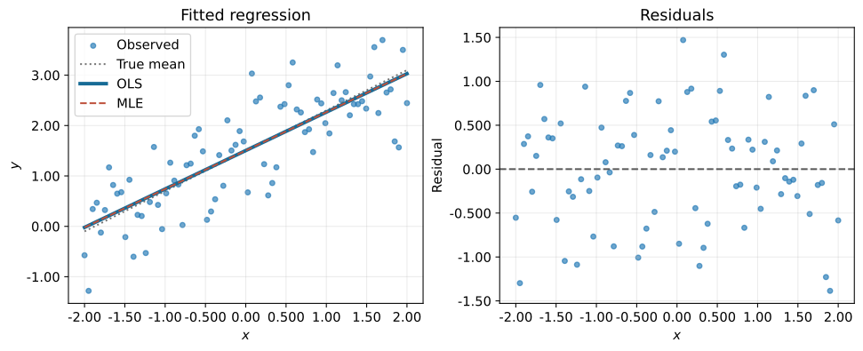
The left plot shows the observations and fitted lines; the right shows the residuals. The OLS and maximum-likelihood lines overlap. A residual plot alone cannot establish normality or independence.
fig, axes = plt.subplots(1, 2, figsize=(10, 4), layout="constrained")
axes[0].scatter(x, y, s=18, alpha=0.650, label="Observed")
axes[0].plot(x, X @ b_true, color="0.450", linestyle=":", label="True mean")
axes[0].plot(x, X @ b_ols, color="#176b96", linewidth=3, label="OLS")
axes[0].plot(x, X @ b_mle, color="#bd503b", linestyle="--", label="MLE")
axes[0].set(xlabel="$x$", ylabel="$y$", title="Fitted regression")
axes[0].legend()
axes[1].scatter(x, residual, s=18, alpha=0.650)
axes[1].axhline(0, color="0.350", linestyle="--")
axes[1].set(xlabel="$x$", ylabel="Residual", title="Residuals")
save_svg(fig, "ols_01_fit_residuals.svg")
Residual sum of squares and log-likelihood
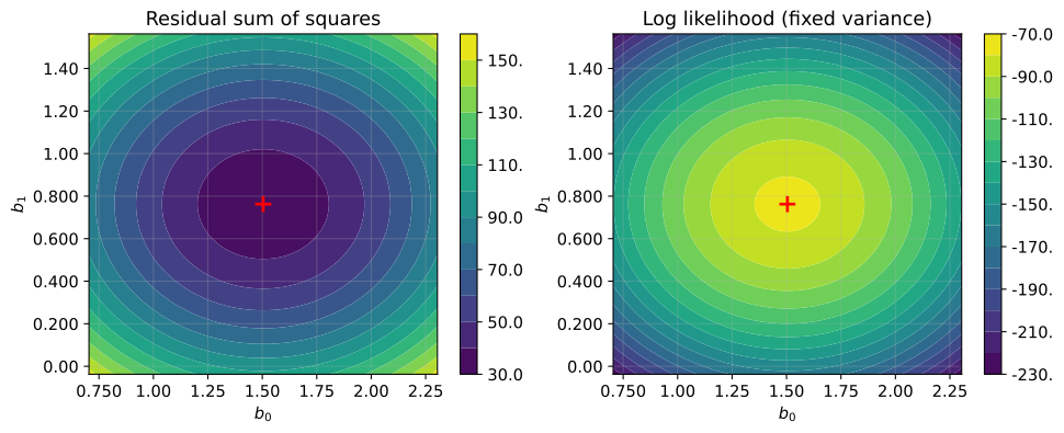
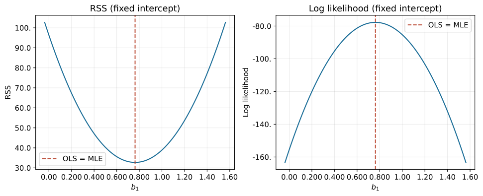
With the variance fixed at its estimate, the minimum on the left and the maximum on the right occur at the same point. The following figure shows a cross section that also fixes the intercept and varies only the slope.
b0_grid = np.linspace(b_ols[0] - 0.800, b_ols[0] + 0.800, 121)
b1_grid = np.linspace(b_ols[1] - 0.800, b_ols[1] + 0.800, 121)
B0, B1 = np.meshgrid(b0_grid, b1_grid)
# Use the last axis for observations and compute the residual sum of squares for each candidate.
grid_residual = y - B0[..., None] - B1[..., None] * x
S_grid = np.sum(grid_residual**2, axis=-1)
ell_grid = -n / 2 * np.log(2 * np.pi * v_mle) - S_grid / (2 * v_mle)

fig, axes = plt.subplots(1, 2, figsize=(10, 4), layout="constrained")
for ax, values, title in zip(axes, [S_grid, ell_grid],
                             ["Residual sum of squares", "Log likelihood (fixed variance)"]):
    contour = ax.contourf(B0, B1, values, levels=14, cmap="viridis")
    ax.plot(*b_ols, "r+", markersize=11, markeredgewidth=2)
    ax.set(xlabel="$b_0$", ylabel="$b_1$", title=title)
    fig.colorbar(contour, ax=ax)
save_svg(fig, "ols_02_contours.svg")

S_slice = np.sum((y - b_ols[0] - b1_grid[:, None] * x)**2, axis=1)
ell_slice = -n / 2 * np.log(2 * np.pi * v_mle) - S_slice / (2 * v_mle)
fig, axes = plt.subplots(1, 2, figsize=(10, 4), layout="constrained")
for ax, values, label in zip(axes, [S_slice, ell_slice], ["RSS", "Log likelihood"]):
    ax.plot(b1_grid, values, color="#176b96")
    ax.axvline(b_ols[1], color="#bd503b", linestyle="--", label="OLS = MLE")
    ax.set(xlabel="$b_1$", ylabel=label, title=label + " (fixed intercept)")
    ax.legend()
save_svg(fig, "ols_03_slope_slice.svg")
Estimating the variance
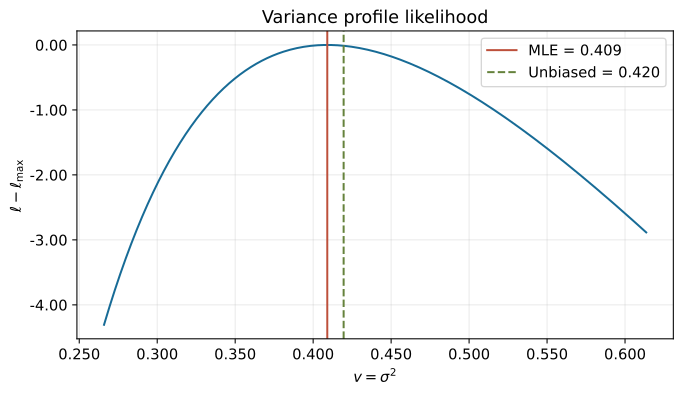
With the coefficients fixed at the OLS solution, the log-likelihood is maximized at $S_*/n$. The unbiased variance estimate $S_*/(n-p)$ differs from this maximum.
v_grid = np.linspace(v_mle * 0.650, v_mle * 1.50, 400)
ell_v = -n / 2 * np.log(2 * np.pi * v_grid) - rss / (2 * v_grid)
ell_max = -negative_log_likelihood(theta_ols)
fig, ax = plt.subplots(figsize=(7, 4), layout="constrained")
ax.plot(v_grid, ell_v - ell_max, color="#176b96")
ax.axvline(v_mle, color="#bd503b", label=f"MLE = {sig3(v_mle)}")
ax.axvline(v_unbiased, color="#65823c", linestyle="--",
           label=f"Unbiased = {sig3(v_unbiased)}")
ax.set(xlabel=r"$v=\sigma^2$", ylabel=r"$\ell-\ell_{\max}$",
       title="Variance profile likelihood")
ax.legend()
save_svg(fig, "ols_04_variance_profile.svg")
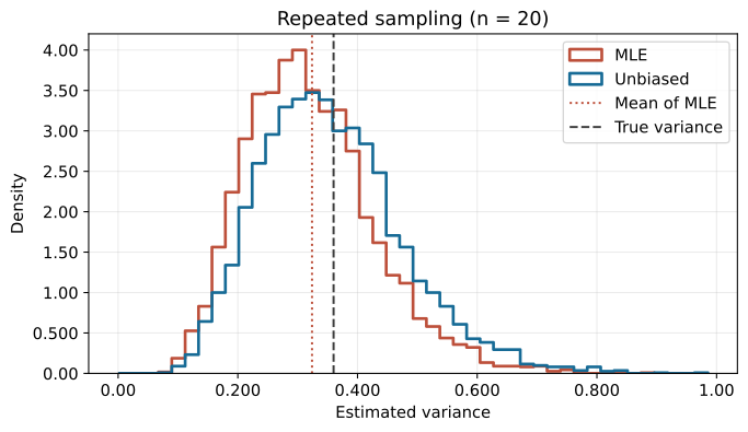
Repeat a regression with 20 observations 5,000 times and compare the average variance estimates. The true variance is $0.360$, and the expected maximum-likelihood estimate is $(18/20)\times0.360=0.324$. The distributions overlap, but the maximum-likelihood estimates have a smaller mean.
sim_rng = np.random.default_rng(102)
n_sim, repeats = 20, 5000
X_sim = np.column_stack([np.ones(n_sim), np.linspace(-2, 2, n_sim)])
# Treat each column as one simulated data set and solve the least-squares problems together.
Y_sim = (X_sim @ b_true)[:, None] + sim_rng.normal(
    0, sigma_true, size=(n_sim, repeats)
)
B_sim = np.linalg.lstsq(X_sim, Y_sim, rcond=None)[0]
R_sim = Y_sim - X_sim @ B_sim
rss_sim = np.sum(R_sim**2, axis=0)
mle_sim = rss_sim / n_sim
unbiased_sim = rss_sim / (n_sim - p)
v_true = sigma_true**2
expected_mle = (n_sim - p) / n_sim * v_true
pprint({"true variance": sig3(v_true), "theoretical MLE mean": sig3(expected_mle),
        "sample MLE mean": sig3(mle_sim.mean()),
        "sample mean of unbiased estimates": sig3(unbiased_sim.mean())})

fig, ax = plt.subplots(figsize=(7, 4), layout="constrained")
bins = np.linspace(0, max(mle_sim.max(), unbiased_sim.max()), 45)
ax.hist(mle_sim, bins=bins, density=True, histtype="step", linewidth=2,
        color="#bd503b", label="MLE")
ax.hist(unbiased_sim, bins=bins, density=True, histtype="step", linewidth=2,
        color="#176b96", label="Unbiased")
ax.axvline(expected_mle, color="#bd503b", linestyle=":", label="Mean of MLE")
ax.axvline(v_true, color="0.250", linestyle="--", label="True variance")
ax.set(xlabel="Estimated variance", ylabel="Density", title="Repeated sampling (n = 20)")
ax.legend()
save_svg(fig, "ols_05_variance_sampling.svg")
{'sample MLE mean': '0.321',
 'theoretical MLE mean': '0.324',
 'sample mean of unbiased estimates': '0.357',
 'true variance': '0.360'}
Conclusion
Assuming independent normal errors with equal variance, we derived OLS and the error-variance estimator from maximum likelihood.
The coefficient-dependent part of the log-likelihood is a negative constant times the residual sum of squares. This makes the maximum-likelihood coefficient estimate equal to the OLS solution. Maximum likelihood divides the residual sum of squares by $n$ to estimate variance, while the unbiased estimator divides by $n-p$. With correlated errors or unequal variances, this likelihood no longer applies as written, and ordinary OLS need not agree with maximum likelihood.