Why are Hilbert matrices difficult for computers? (Rewritten from an earlier blog post)
Environment
Python 3.14.6, NumPy 2.5.4, SciPy 1.18.1, mpmath 1.3.0, Matplotlib 3.11.2 (Jupyter Notebook).
This article is a rewrite of a post from around 2013–2016, with calculations performed in the environment described above.
Overview
A Hilbert matrix has an inverse. However, in a linear system with this coefficient matrix, a small error in the input can cause a large change in the solution.
We first show that Hilbert matrices are invertible and use the condition number to explain error amplification. We then use Python to compare residuals with solution errors, examine how changes to the right-hand side affect the solution, and test different calculation precisions.
Setup
Run the code in Jupyter Notebook from top to bottom. Round numbers to three significant digits only when displaying them.
import sys
from pathlib import Path
from pprint import pprint

import matplotlib
import matplotlib.pyplot as plt
import mpmath as mp
import numpy as np
import scipy
from IPython.display import Math, display
from matplotlib.ticker import FuncFormatter, MaxNLocator
from matplotlib_inline.backend_inline import set_matplotlib_formats
from scipy.linalg import hilbert

%matplotlib inline

print(f"Python: {sys.version.split()[0]}")
print(f"NumPy {np.__version__}, SciPy {scipy.__version__}")
print(f"Matplotlib {matplotlib.__version__}, mpmath {mp.__version__}")

# Round numbers to three significant digits only for display.
# .2e uses two decimal places in scientific notation, giving three significant digits.
np.set_printoptions(formatter={"float_kind": lambda value: f"{value:.2e}"})
tick_formatter = FuncFormatter(lambda value, position: f"{value:#.3g}")

# Embed figures in the notebook in SVG format.
set_matplotlib_formats("svg")
plt.rcParams.update({
    "figure.figsize": (11, 4),
    "figure.dpi": 130,
    "savefig.format": "svg",
    "font.size": 10,
    "axes.grid": True,
    "grid.alpha": 0.250,
})


# Create a directory for SVG files under the current working directory.
figure_dir = Path("figures")
figure_dir.mkdir(parents=True, exist_ok=True)


def scientific_latex(value):
    """Convert a number to LaTeX notation with three significant digits."""
    mantissa, exponent = f"{float(value):.2e}".split("e")
    return rf"{mantissa}\times 10^{{{int(exponent)}}}"


def make_mp_hilbert(size):
    """Build a Hilbert matrix at the current mpmath precision."""
    # Convert integers to mpmath numbers before division to avoid double-precision rounding.
    # Python indices start at zero, so the denominator is i + j + 1.
    return mp.matrix([
        [mp.mpf(1) / (i + j + 1) for j in range(size)]
        for i in range(size)
    ])
Python: 3.14.6
NumPy 2.5.4, SciPy 1.18.1
Matplotlib 3.11.2, mpmath 1.3.0
1. Definition and invertibility of the Hilbert matrix
Formulas and reasoning
Using indices that start at one, the Hilbert matrix $\mathbf{H}_n$ of size $n$ is defined as follows. Python indices start at zero, so the implementation uses i + j + 1 in the denominator. The official SciPy documentation gives the same definition.
$$ \begin{aligned} \mathbf{H}_n&=(h_{ij}),\qquad h_{ij}=\frac{1}{i+j-1},\\ &\quad 1\le i,j\le n. \end{aligned} $$
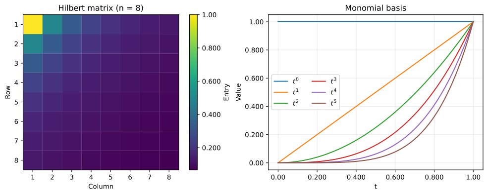
Each entry can also be written as the integral of a product of monomials over $[0,1]$.
$$ \begin{aligned} \int_0^1 t^{i-1}t^{j-1}\,dt &=\int_0^1 t^{i+j-2}\,dt\\ &=\left[\frac{t^{i+j-1}}{i+j-1}\right]_0^1\\ &=\frac{1}{i+j-1}. \end{aligned} $$
For any real vector $\mathbf{c}\ne\mathbf{0}$, exchanging the sum and integral gives
$$ \begin{aligned} \mathbf{c}^{\mathsf T}\mathbf{H}_n\mathbf{c} &=\sum_{i=1}^n\sum_{j=1}^n c_i c_j h_{ij}\\ &=\int_0^1\sum_{i=1}^n\sum_{j=1}^n c_i c_j t^{i-1}t^{j-1}\,dt\\ &=\int_0^1\left(\sum_{i=1}^n c_i t^{i-1}\right)^2dt>0. \end{aligned} $$
If $\mathbf{c}\ne\mathbf{0}$, this polynomial is not identically zero, so the integral of its square is positive. Thus, $\mathbf{H}_n$ is symmetric positive definite and therefore invertible.
In a linear combination of monomials, terms can cancel, making the integral of the square small even when the coefficient vector has Euclidean norm one. The minimum of $\mathbf{c}^{\mathsf T}\mathbf{H}_n\mathbf{c}$ over all unit vectors is the smallest eigenvalue of $\mathbf{H}_n$. Thus, a unit vector that gives a small integral also implies a small minimum eigenvalue.
Python example
# Display the 3-by-3 matrix using both decimals and fractions.
H3 = hilbert(3)
print("Hilbert matrix (n = 3, decimal values)")
pprint(H3)

# Render formulas as LaTeX instead of printing them as strings.
display(
    Math(
        r"\mathbf{H}_3=\begin{bmatrix}"
        r"1 & \frac{1}{2} & \frac{1}{3}\\"
        r"\frac{1}{2} & \frac{1}{3} & \frac{1}{4}\\"
        r"\frac{1}{3} & \frac{1}{4} & \frac{1}{5}"
        r"\end{bmatrix}"
    )
)
Hilbert matrix (n = 3, decimal values)
array([[1.00e+00, 5.00e-01, 3.33e-01],
       [5.00e-01, 3.33e-01, 2.50e-01],
       [3.33e-01, 2.50e-01, 2.00e-01]])
$$ \displaystyle \mathbf{H}_3=\begin{bmatrix}1 & \frac{1}{2} & \frac{1}{3}\\\frac{1}{2} & \frac{1}{3} & \frac{1}{4}\\\frac{1}{3} & \frac{1}{4} & \frac{1}{5}\end{bmatrix} $$
fig, axes = plt.subplots(1, 2, layout="constrained")

# Left: use color to show entry values, with row and column numbers starting at one.
# Draw each entry as a rectangle to retain vector graphics in the SVG.
cell_edges = np.arange(9) + 0.500
heatmap = axes[0].pcolormesh(
    cell_edges,
    cell_edges,
    hilbert(8),
    cmap="viridis",
    shading="flat",
    edgecolors="face",
    linewidth=0.100,
)
axes[0].set_aspect("equal")
axes[0].invert_yaxis()
axes[0].grid(False)
axes[0].set(title="Hilbert matrix (n = 8)", xlabel="Column", ylabel="Row")
axes[0].set_xticks(range(1, 9))
axes[0].set_yticks(range(1, 9))
colorbar = fig.colorbar(heatmap, ax=axes[0], format=tick_formatter, label="Entry")
# Save the color bar as vector graphics too.
colorbar.solids.set_rasterized(False)
# Prevent white seams between color regions in the SVG display.
colorbar.solids.set_edgecolor("face")

# Right: plot the monomials that appear in the integral expression for the entries.
t = np.linspace(0, 1, 300)
for degree in range(6):
    axes[1].plot(t, t**degree, label=rf"$t^{degree}$")

axes[1].set(title="Monomial basis", xlabel="t", ylabel="Value")
axes[1].xaxis.set_major_formatter(tick_formatter)
axes[1].yaxis.set_major_formatter(tick_formatter)
axes[1].legend(ncol=2)
# Save as an SVG file and display it in the notebook.
svg_path = figure_dir / "01_hilbert_and_monomials.svg"
fig.savefig(svg_path, format="svg", bbox_inches="tight")
print(f"SVG saved to: {svg_path.as_posix()}")
plt.show()
SVG saved to: figures/01_hilbert_and_monomials.svg
2. Condition numbers and error amplification
Formulas and reasoning
Write $\mathbf{H}=\mathbf{H}_n$ for short. We use the Euclidean vector norm and its corresponding matrix 2-norm. If the largest and smallest singular values are $\sigma_{\max}$ and $\sigma_{\min}$, the condition number is
$$ \kappa_2(\mathbf{H})=\|\mathbf{H}\|_2\|\mathbf{H}^{-1}\|_2 =\frac{\sigma_{\max}}{\sigma_{\min}} $$
Assume $\mathbf{b}\ne\mathbf{0}$. Keep the matrix $\mathbf{H}$ fixed and change only the right-hand side.
$$ \begin{aligned} \mathbf{H}\mathbf{x}&=\mathbf{b},\\ \mathbf{H}(\mathbf{x}+\Delta\mathbf{x})&=\mathbf{b}+\Delta\mathbf{b},\\ \mathbf{H}\Delta\mathbf{x}&=\Delta\mathbf{b},\\ \Delta\mathbf{x}&=\mathbf{H}^{-1}\Delta\mathbf{b}. \end{aligned} $$
We have $\|\Delta\mathbf{x}\|_2\le\|\mathbf{H}^{-1}\|_2\|\Delta\mathbf{b}\|_2$ and $\|\mathbf{b}\|_2\le\|\mathbf{H}\|_2\|\mathbf{x}\|_2$. Combining these gives the following inequality.
$$ \begin{aligned} \frac{\|\Delta\mathbf{x}\|_2}{\|\mathbf{x}\|_2} &\le\|\mathbf{H}^{-1}\|_2\|\Delta\mathbf{b}\|_2 \frac{\|\mathbf{H}\|_2}{\|\mathbf{b}\|_2} \\ &=\kappa_2(\mathbf{H})\frac{\|\Delta\mathbf{b}\|_2}{\|\mathbf{b}\|_2}. \end{aligned} $$
This inequality shows that the relative error in the solution is at most the condition number times the relative error in the right-hand side. The actual amplification depends on the directions of the original right-hand side and the added error.
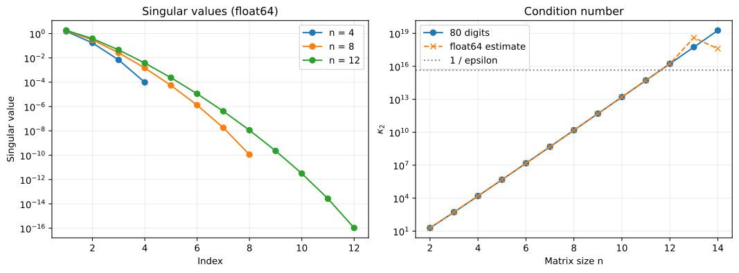
The following code compares condition numbers obtained by a double-precision singular value decomposition with those computed at 80 decimal digits of precision. For a symmetric positive definite matrix, eigenvalues and singular values coincide, so the high-precision calculation uses the ratio of the largest and smallest eigenvalues.
Python example
matrix_sizes = np.arange(2, 15)
condition_float64 = []
condition_high_precision = []

for size in matrix_sizes:
    size = int(size)

    # Use a singular value decomposition to compute the 2-norm condition number in double precision.
    condition_float64.append(np.linalg.cond(hilbert(size), 2))

    # For a symmetric positive definite matrix, the ratio of extreme eigenvalues also gives the condition number.
    with mp.workdps(80):
        eigenvalues = mp.eigsy(make_mp_hilbert(size), eigvals_only=True)
        condition = eigenvalues[size - 1] / eigenvalues[0]

        # Convert to float for display and plotting only after computing the condition number.
        condition_high_precision.append(float(condition))

condition_float64 = np.array(condition_float64)
condition_high_precision = np.array(condition_high_precision)

# Print selected matrix sizes to make the changes easier to read.
condition_summary = []
for size, value64, value80 in zip(matrix_sizes, condition_float64, condition_high_precision):
    if size in (6, 10, 12, 14):
        condition_summary.append(
            {
                "n": int(size),
                "cond_float64": f"{value64:.2e}",
                "cond_80digits": f"{value80:.2e}",
            }
        )

print("Condition numbers by matrix size (double precision and 80 digits)")
pprint(condition_summary, sort_dicts=False)
Condition numbers by matrix size (double precision and 80 digits)
[{'n': 6, 'cond_float64': '1.50e+07', 'cond_80digits': '1.50e+07'},
 {'n': 10, 'cond_float64': '1.60e+13', 'cond_80digits': '1.60e+13'},
 {'n': 12, 'cond_float64': '1.72e+16', 'cond_80digits': '1.71e+16'},
 {'n': 14, 'cond_float64': '4.05e+17', 'cond_80digits': '1.85e+19'}]
fig, axes = plt.subplots(1, 2, layout="constrained")

# Left: use a logarithmic vertical axis to compare even the small singular values.
for size in (4, 8, 12):
    singular_values = np.linalg.svd(hilbert(size), compute_uv=False)
    indices = np.arange(1, size + 1)
    axes[0].semilogy(indices, singular_values, "o-", label=f"n = {size}")

axes[0].set(
    title="Singular values (float64)",
    xlabel="Index",
    ylabel="Singular value",
)
axes[0].xaxis.set_major_locator(MaxNLocator(integer=True))
axes[0].legend()

# Right: compare double-precision and high-precision condition numbers at the same sizes.
axes[1].semilogy(matrix_sizes, condition_high_precision, "o-", label="80 digits")
axes[1].semilogy(matrix_sizes, condition_float64, "x--", label="float64 estimate")
axes[1].axhline(
    1 / np.finfo(float).eps,
    color="gray",
    linestyle=":",
    label="1 / epsilon",
)
axes[1].set(title="Condition number", xlabel="Matrix size n", ylabel=r"$\kappa_2$")
axes[1].xaxis.set_major_locator(MaxNLocator(integer=True))
axes[1].legend()
# Save as an SVG file and display it in the notebook.
svg_path = figure_dir / "02_singular_values_and_condition.svg"
fig.savefig(svg_path, format="svg", bbox_inches="tight")
print(f"SVG saved to: {svg_path.as_posix()}")
plt.show()
SVG saved to: figures/02_singular_values_and_condition.svg
Results
For $n=14$, the 80-digit condition number is about $1.85\times10^{19}$. Double precision in this environment gives about $4.05\times10^{17}$, showing that even the condition number itself is computed with error.
3. Rounding errors and small residuals
Formulas and reasoning
The gap between 1 and the next larger number representable in float64 is $\varepsilon=2^{-52}\approx2.22\times10^{-16}$. For rounding to nearest, the unit roundoff is $u=\varepsilon/2$. Numbers such as $1/3$ cannot be represented exactly with finitely many binary digits, so storing them introduces rounding error. Higham’s explanation also discusses this input error and the tendency to amplify errors, known as ill-conditioning.
Computing $\kappa_2(\mathbf{H}_{12})$ at 80 digits gives about $1.71\times10^{16}$. At this scale, double-precision rounding errors can be amplified enough to destroy significant digits in the solution. For larger matrices, even a condition number computed in double precision can have a large error.
Double-precision results depend on the execution environment. For large condition numbers, differences can affect leading digits, not just the last few digits.
Set the reference solution to $\mathbf{x}_*=\mathbf{1}$, compute $\mathbf{b}=\mathbf{H}\mathbf{x}_*$, and solve the linear system. Here, $\mathbf{1}$ is the vector whose entries are all one. In the code, however, rounding occurs both when storing the matrix and when forming the right-hand side by matrix-vector multiplication. Let $\widehat{\mathbf{x}}$ be the computed solution. Define the relative forward error $E$ against the reference solution and the relative residual $R$ as follows.
$$ E=\frac{\|\widehat{\mathbf{x}}-\mathbf{x}_*\|_2}{\|\mathbf{x}_*\|_2}, \qquad R=\frac{\|\mathbf{b}-\mathbf{H}\widehat{\mathbf{x}}\|_2}{\|\mathbf{b}\|_2}. $$
For inputs $\mathbf{H},\mathbf{b}$, let $\mathbf{x}$ be the exact solution and let $\mathbf{r}=\mathbf{b}-\mathbf{H}\widehat{\mathbf{x}}$ be the residual. Then
$$ \mathbf{r}=\mathbf{H}(\mathbf{x}-\widehat{\mathbf{x}}),\qquad \widehat{\mathbf{x}}-\mathbf{x}=-\mathbf{H}^{-1}\mathbf{r}. $$
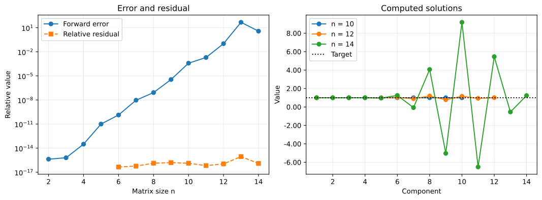
The same argument as in the previous section bounds the relative forward error against the exact solution $\mathbf{x}$ by $\kappa_2(\mathbf{H})R$. With a large condition number, this bound can be large even for a small residual, so the residual alone cannot establish solution accuracy.
This bound uses the exact solution $\mathbf{x}$ for the same inputs as its reference. In contrast, the experimental error $E$ uses $\mathbf{x}_*$ as its reference, so it also includes the effect of rounding the inputs. The residual is itself computed in double precision and also contains rounding error. Residuals computed as zero are omitted from logarithmic axes.
Python example
forward_errors = []
relative_residuals = []
computed_solutions = {}

for size in matrix_sizes:
    size = int(size)
    H = hilbert(size)

    # Use an all-ones target solution and form its right-hand side.
    # This matrix-vector product also introduces double-precision rounding.
    x_true = np.ones(size)
    b = H @ x_true
    x_hat = np.linalg.solve(H, b)

    # Evaluate solution error separately from how closely the equations are satisfied.
    forward_error = np.linalg.norm(x_hat - x_true) / np.linalg.norm(x_true)
    relative_residual = np.linalg.norm(b - H @ x_hat) / np.linalg.norm(b)

    forward_errors.append(forward_error)
    relative_residuals.append(relative_residual)
    computed_solutions[size] = x_hat

error_summary = []
for size, error, residual in zip(matrix_sizes, forward_errors, relative_residuals):
    if size in (8, 10, 12, 14):
        error_summary.append(
            {
                "n": int(size),
                "forward_error": f"{error:.2e}",
                "relative_residual": f"{residual:.2e}",
            }
        )

print("Relative forward errors and relative residuals")
pprint(error_summary, sort_dicts=False)
display(Math(r"\varepsilon=" + scientific_latex(np.finfo(float).eps)))
Relative forward errors and relative residuals
[{'n': 8, 'forward_error': '8.31e-08', 'relative_residual': '1.34e-16'},
 {'n': 10, 'forward_error': '3.81e-04', 'relative_residual': '1.31e-16'},
 {'n': 12, 'forward_error': '1.03e-01', 'relative_residual': '1.09e-16'},
 {'n': 14, 'forward_error': '3.71e+00', 'relative_residual': '1.24e-16'}]
$$ \displaystyle \varepsilon=2.22\times 10^{-16} $$
fig, axes = plt.subplots(1, 2, layout="constrained")

# Left: omit residuals computed as zero because a logarithmic axis cannot display them.
# np.nan marks missing plot values; it does not change the computed residuals.
positive_residuals = np.where(
    np.array(relative_residuals) > 0,
    relative_residuals,
    np.nan,
)
axes[0].semilogy(matrix_sizes, forward_errors, "o-", label="Forward error")
axes[0].semilogy(matrix_sizes, positive_residuals, "s--", label="Relative residual")
axes[0].set(
    title="Error and residual",
    xlabel="Matrix size n",
    ylabel="Relative value",
)
axes[0].xaxis.set_major_locator(MaxNLocator(integer=True))
axes[0].legend()

# Right: compare each component of the computed solution with the target value of one.
for size in (10, 12, 14):
    indices = np.arange(1, size + 1)
    axes[1].plot(indices, computed_solutions[size], "o-", label=f"n = {size}")

axes[1].axhline(1, color="black", linestyle=":", label="Target")
axes[1].set(title="Computed solutions", xlabel="Component", ylabel="Value")
axes[1].xaxis.set_major_locator(MaxNLocator(integer=True))
axes[1].yaxis.set_major_formatter(tick_formatter)
axes[1].legend()
# Save as an SVG file and display it in the notebook.
svg_path = figure_dir / "03_errors_and_solutions.svg"
fig.savefig(svg_path, format="svg", bbox_inches="tight")
print(f"SVG saved to: {svg_path.as_posix()}")
plt.show()
SVG saved to: figures/03_errors_and_solutions.svg
Results
For $n=12$ in this environment, the relative residual is $1.09\times10^{-16}$, while the relative forward error is $1.03\times10^{-1}$. Although the residual is comparable to machine epsilon $\varepsilon$, the relative difference from the reference solution is about 10%.
4. Making a small change to the right-hand side
Formulas and reasoning
The left singular vectors $\mathbf{u}_i$ and right singular vectors $\mathbf{v}_i$ are unit vectors satisfying $\mathbf{H}\mathbf{v}_i=\sigma_i\mathbf{u}_i$. Set $\mathbf{x}=\mathbf{v}_{\max}$ and $\mathbf{b}=\sigma_{\max}\mathbf{u}_{\max}$, and for $\delta>0$ add $\Delta\mathbf{b}=\delta\sigma_{\max}\mathbf{u}_{\min}$. The relative change in the right-hand side is $\delta$, and the solution changes as follows.
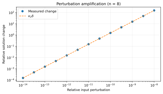
$$ \begin{aligned} \Delta\mathbf{x} &=\mathbf{H}^{-1}\Delta\mathbf{b} =\frac{\delta\sigma_{\max}}{\sigma_{\min}}\mathbf{v}_{\min},\\ \frac{\|\Delta\mathbf{x}\|_2}{\|\mathbf{x}\|_2} &=\delta\kappa_2(\mathbf{H}). \end{aligned} $$
With these choices of the original solution and perturbation direction, the relative amplification equals the condition number. The next code uses $n=8$ and compares the relative changes in the right-hand side and solution. Both the original and perturbed solutions are computed numerically, so rounding errors can cause deviations from theory when the input change is extremely small.
Python example
H = hilbert(8)
U, singular_values, Vt = np.linalg.svd(H)

# Choose the right singular vector for the largest singular value as the original solution.
x_original = Vt[0]
b_original = H @ x_original
x_baseline = np.linalg.solve(H, b_original)

perturbation_sizes = np.logspace(-14, -8, 13)
relative_changes = []

for delta in perturbation_sizes:
    # Perturb the right-hand side along the left singular vector for the smallest singular value.
    # Set the perturbation norm to delta times the norm of the original right-hand side.
    delta_b = delta * np.linalg.norm(b_original) * U[:, -1]
    x_shifted = np.linalg.solve(H, b_original + delta_b)

    relative_change = np.linalg.norm(x_shifted - x_baseline) / np.linalg.norm(x_baseline)
    relative_changes.append(relative_change)

condition_number = singular_values[0] / singular_values[-1]
theoretical_changes = condition_number * perturbation_sizes

# Also check agreement with theory in a numerical table.
perturbation_summary = []
for index in (0, 6, 12):
    perturbation_summary.append(
        {
            "input_change": f"{perturbation_sizes[index]:.2e}",
            "solution_change": f"{relative_changes[index]:.2e}",
            "theory": f"{theoretical_changes[index]:.2e}",
        }
    )

print("Relative changes in the input and solution")
pprint(perturbation_summary, sort_dicts=False)
Relative changes in the input and solution
[{'input_change': '1.00e-14',
  'solution_change': '1.52e-04',
  'theory': '1.53e-04'},
 {'input_change': '1.00e-11',
  'solution_change': '1.53e-01',
  'theory': '1.53e-01'},
 {'input_change': '1.00e-08',
  'solution_change': '1.53e+02',
  'theory': '1.53e+02'}]
# Compare measured changes with the condition-number prediction on log-log axes.
fig, ax = plt.subplots(figsize=(7, 4), layout="constrained")
ax.loglog(perturbation_sizes, relative_changes, "o", label="Measured change")
ax.loglog(
    perturbation_sizes,
    theoretical_changes,
    "--",
    label=r"$\kappa_2\delta$",
)
ax.set(
    title="Perturbation amplification (n = 8)",
    xlabel="Relative input perturbation",
    ylabel="Relative solution change",
)
ax.legend()
# Save as an SVG file and display it in the notebook.
svg_path = figure_dir / "04_perturbation_amplification.svg"
fig.savefig(svg_path, format="svg", bbox_inches="tight")
print(f"SVG saved to: {svg_path.as_posix()}")
plt.show()
SVG saved to: figures/04_perturbation_amplification.svg
5. What to check when increasing precision
Formulas and reasoning
The function np.linalg.solve solves a linear system without explicitly forming an inverse, but it does not change the problem’s condition number. To improve the solution accuracy for the original Hilbert matrix, each entry $1/(i+j-1)$ and the right-hand side must be recomputed at high precision. Converting a matrix and right-hand side that have already been rounded to double precision cannot recover the lost information.
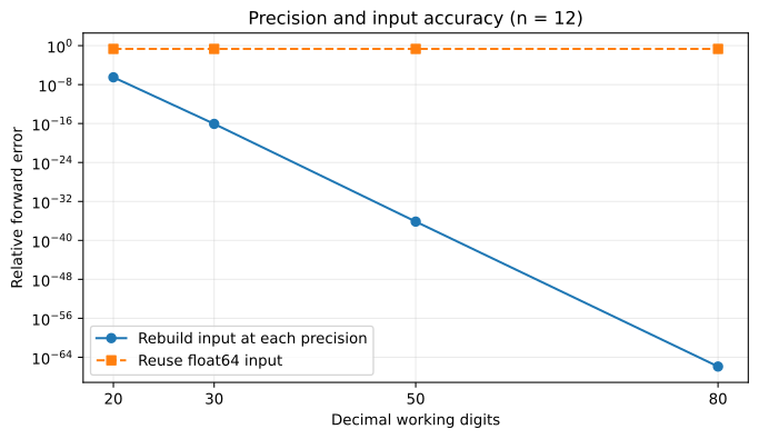
In the next comparison, fix $n=12$. One approach rebuilds the matrix and right-hand side at each precision; the other converts the existing double-precision inputs to high precision. Both measure relative forward error against the all-ones reference solution. The second approach accurately solves the system with rounded inputs, whose solution differs from the reference.
Python example
size = 12
H_float64 = hilbert(size)
b_float64 = H_float64 @ np.ones(size)

working_digits = [20, 30, 50, 80]
rebuilt_input_errors = []
rounded_input_errors = []

for digits in working_digits:
    with mp.workdps(digits):
        x_true = mp.matrix([1] * size)

        # Method 1: rebuild the matrix and right-hand side at the current high precision.
        H_rebuilt = make_mp_hilbert(size)
        b_rebuilt = H_rebuilt * x_true
        x_rebuilt = mp.lu_solve(H_rebuilt, b_rebuilt)

        # Method 2: convert inputs already rounded to double precision to high precision.
        # More calculation digits cannot recover information lost when forming the inputs.
        H_rounded = mp.matrix(H_float64.tolist())
        b_rounded = mp.matrix(b_float64.tolist())
        x_rounded = mp.lu_solve(H_rounded, b_rounded)

        # Evaluate errors at high precision, then convert to float for display and plotting.
        rebuilt_error = mp.norm(x_rebuilt - x_true) / mp.norm(x_true)
        rounded_error = mp.norm(x_rounded - x_true) / mp.norm(x_true)
        rebuilt_input_errors.append(float(rebuilt_error))
        rounded_input_errors.append(float(rounded_error))

precision_summary = []
for digits, rebuilt_error, rounded_error in zip(working_digits, rebuilt_input_errors, rounded_input_errors):
    precision_summary.append(
        {
            "digits": digits,
            "rebuilt_input_error": f"{rebuilt_error:.2e}",
            "float64_input_error": f"{rounded_error:.2e}",
        }
    )

print("Relative forward errors by input construction and calculation precision")
pprint(precision_summary, sort_dicts=False)
Relative forward errors by input construction and calculation precision
[{'digits': 20,
  'rebuilt_input_error': '3.15e-07',
  'float64_input_error': '2.11e-01'},
 {'digits': 30,
  'rebuilt_input_error': '8.44e-17',
  'float64_input_error': '2.11e-01'},
 {'digits': 50,
  'rebuilt_input_error': '7.19e-37',
  'float64_input_error': '2.11e-01'},
 {'digits': 80,
  'rebuilt_input_error': '1.23e-66',
  'float64_input_error': '2.11e-01'}]
# Compare the number of high-precision digits with the difference from the target solution.
fig, ax = plt.subplots(figsize=(7, 4), layout="constrained")
ax.semilogy(
    working_digits,
    rebuilt_input_errors,
    "o-",
    label="Rebuild input at each precision",
)
ax.semilogy(
    working_digits,
    rounded_input_errors,
    "s--",
    label="Reuse float64 input",
)
ax.set(
    title="Precision and input accuracy (n = 12)",
    xlabel="Decimal working digits",
    ylabel="Relative forward error",
)
ax.set_xticks(working_digits)
ax.legend()
# Save as an SVG file and display it in the notebook.
svg_path = figure_dir / "05_precision_and_input_accuracy.svg"
fig.savefig(svg_path, format="svg", bbox_inches="tight")
print(f"SVG saved to: {svg_path.as_posix()}")
plt.show()
SVG saved to: figures/05_precision_and_input_accuracy.svg
Results
When the inputs are rebuilt at 80 digits, the relative forward error against the reference is about $1.23\times10^{-66}$. Reusing double-precision inputs gives about $2.11\times10^{-1}$, and increasing calculation precision does not remove the difference from the reference.
Conclusion
Linear systems with Hilbert coefficient matrices have large condition numbers. Small input and calculation errors are amplified, making accurate solutions difficult to obtain in double precision.
An inverse can exist without finite-precision calculations giving an accurate solution. Check both the residual and the condition number, and increase precision from the input-construction stage if needed. When a Hilbert matrix arises in polynomial approximation, using an orthogonal basis instead of monomials is another option.