Why does the condition number describe numerical difficulty? (Rewritten from an earlier blog post)
Environment
Python 3.14.6, NumPy 2.5.4, Matplotlib 3.11.2 (Jupyter Notebook).
This article is a rewrite of a post from around 2013–2016, with calculations performed in the environment described above.
Overview
With the coefficient matrix of a linear system fixed, the relative error in the solution is at most the matrix condition number times the relative error in the right-hand side. Suitable directions for the right-hand side and the error can attain this bound.
We derive this bound and use Python to examine the relation between singular values and condition numbers, the effect of error direction on amplification, and the difference between residuals and solution errors. Here, “difficulty” means that a small input error can have a large effect on solution accuracy.
Setup
Run the code in Jupyter Notebook from top to bottom. Round numbers to three significant digits only when displaying them.
import sys
from pathlib import Path
from pprint import pprint

import matplotlib
import matplotlib.pyplot as plt
import numpy as np
from IPython.display import Math, display
from matplotlib.ticker import FuncFormatter, NullFormatter
from matplotlib_inline.backend_inline import set_matplotlib_formats

%matplotlib inline

print(f"Python: {sys.version.split()[0]}")
print(f"NumPy: {np.__version__}, Matplotlib: {matplotlib.__version__}")

# Format array values and plot ticks with three significant digits only for display.
np.set_printoptions(formatter={"float_kind": lambda value: f"{value:.2e}"})
tick_formatter = FuncFormatter(lambda value, position: f"{value:#.3g}")
set_matplotlib_formats("svg")
plt.rcParams.update({
    "figure.figsize": (7, 4),
    "font.size": 10,
    "axes.grid": True,
    "grid.alpha": 0.250,
    "savefig.format": "svg",
    "svg.fonttype": "none",
})
figure_dir = Path("figures")
figure_dir.mkdir(parents=True, exist_ok=True)


def latex_number(value):
    """Convert a number to LaTeX notation with three significant digits."""
    mantissa, exponent = f"{float(value):.2e}".split("e")
    return rf"{mantissa}\times 10^{{{int(exponent)}}}"


def save_figure(fig, filename):
    """Format tick labels, save as SVG, and display the figure in the notebook."""
    for ax in fig.axes:
        for axis in (ax.xaxis, ax.yaxis):
            if axis.get_scale() == "linear":
                axis.set_major_formatter(tick_formatter)
            # Show logarithmic ticks as integer powers and hide minor tick labels.
            axis.set_minor_formatter(NullFormatter())
    output_path = figure_dir / filename
    fig.savefig(output_path, format="svg", bbox_inches="tight")
    print(f"SVG saved to: {output_path.as_posix()}")
    plt.show()
Python: 3.14.6
NumPy: 2.5.4, Matplotlib: 3.11.2
1. Deriving the condition number from relative errors
Let $\mathbf{A}$ be a real invertible square matrix, with $\mathbf{A}\mathbf{x}=\mathbf{b}$ and $\mathbf{b}\ne\mathbf{0}$. We use the Euclidean vector norm and its corresponding matrix 2-norm.
$$ \begin{aligned} \|\mathbf{v}\|_2&=\sqrt{\sum_i v_i^2},\\ \|\mathbf{A}\|_2&=\max_{\mathbf{v}\ne\mathbf{0}} \frac{\|\mathbf{A}\mathbf{v}\|_2}{\|\mathbf{v}\|_2}. \end{aligned} $$
First keep the matrix fixed and add a change $\Delta\mathbf{b}$ to the right-hand side. Writing the new solution as $\mathbf{x}+\Delta\mathbf{x}$ gives
$$ \begin{aligned} \mathbf{A}(\mathbf{x}+\Delta\mathbf{x})&=\mathbf{b}+\Delta\mathbf{b},\\ \mathbf{A}\mathbf{x}+\mathbf{A}\Delta\mathbf{x}&=\mathbf{b}+\Delta\mathbf{b},\\ \mathbf{A}\Delta\mathbf{x}&=\Delta\mathbf{b},\\ \Delta\mathbf{x}&=\mathbf{A}^{-1}\Delta\mathbf{b},\\ \|\Delta\mathbf{x}\|_2&\le\|\mathbf{A}^{-1}\|_2\|\Delta\mathbf{b}\|_2. \end{aligned} $$
We also have $\|\mathbf{b}\|_2=\|\mathbf{A}\mathbf{x}\|_2\le\|\mathbf{A}\|_2\|\mathbf{x}\|_2$. This gives the following relative error bound.
$$ \begin{aligned} \frac{\|\Delta\mathbf{x}\|_2}{\|\mathbf{x}\|_2} &\le\frac{\|\mathbf{A}^{-1}\|_2\|\Delta\mathbf{b}\|_2}{\|\mathbf{x}\|_2}\\ &\le\|\mathbf{A}^{-1}\|_2\|\mathbf{A}\|_2 \frac{\|\Delta\mathbf{b}\|_2}{\|\mathbf{b}\|_2}. \end{aligned} $$
The factor $\|\mathbf{A}^{-1}\|_2\|\mathbf{A}\|_2$ in this inequality is the matrix condition number in the 2-norm.
$$ \boxed{\kappa_2(\mathbf{A})=\|\mathbf{A}\|_2\|\mathbf{A}^{-1}\|_2}. $$
$$ \frac{\|\Delta\mathbf{x}\|_2}{\|\mathbf{x}\|_2} \le\kappa_2(\mathbf{A})\frac{\|\Delta\mathbf{b}\|_2}{\|\mathbf{b}\|_2}. $$
When only the right-hand side changes and the matrix stays fixed, this bound holds even for changes that are not small. The condition number is the largest amplification attainable by choosing the directions of $\mathbf{b}$ and $\Delta\mathbf{b}$. This bound is also given in Driscoll and Braun’s textbook.
2. Singular values and changes in shape
Write the singular value decomposition as $\mathbf{A}=\mathbf{U}\mathbf{\Sigma}\mathbf{V}^{\mathsf T}$. The matrices $\mathbf{U},\mathbf{V}$ are orthogonal and preserve vector lengths. The diagonal matrix $\mathbf{\Sigma}$ has positive singular values on its diagonal. If the largest and smallest singular values are $\sigma_{\max}$ and $\sigma_{\min}$, then
$$ \begin{aligned} \|\mathbf{A}\|_2&=\sigma_{\max},\\ \mathbf{A}^{-1}&=\mathbf{V}\mathbf{\Sigma}^{-1}\mathbf{U}^{\mathsf T},\\ \|\mathbf{A}^{-1}\|_2&=\max_i\frac{1}{\sigma_i}=\frac{1}{\sigma_{\min}},\\ \kappa_2(\mathbf{A})&=\frac{\sigma_{\max}}{\sigma_{\min}}\ge1. \end{aligned} $$
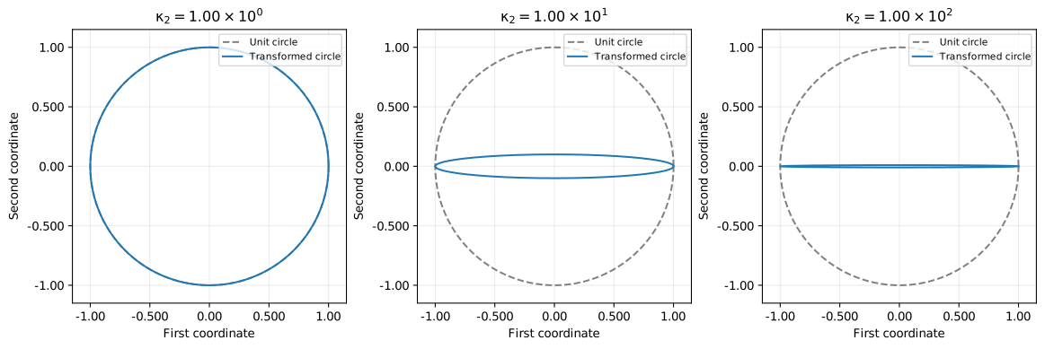
In two dimensions, the matrix $\mathbf{A}$ maps the unit circle to an ellipse. The major and minor semiaxes have lengths $\sigma_{\max}$ and $\sigma_{\min}$. To map the ellipse back to the unit circle, the inverse $\mathbf{A}^{-1}$ scales vectors along the minor axis by $1/\sigma_{\min}$. The condition number is the ratio of the major to minor semiaxis lengths. A singular matrix is defined to have an infinite condition number.
Python example
By default, np.linalg.cond computes the 2-norm condition number using a singular value decomposition; see the official NumPy documentation.
# For a diagonal matrix, the singular values are the absolute values of the diagonal entries.
A = np.diag([1, 0.0100])
singular_values = np.linalg.svd(A, compute_uv=False)
kappa = np.linalg.cond(A)
print("Singular values (descending order)")
pprint(singular_values)
display(Math(
    rf"\kappa_2(\mathbf{{A}})="
    rf"\frac{{{latex_number(singular_values[0])}}}"
    rf"{{{latex_number(singular_values[-1])}}}={latex_number(kappa)}"
))

# Transform the same unit circle using matrices with different condition numbers.
theta = np.linspace(0, 2 * np.pi, 721)
unit_circle = np.vstack([np.cos(theta), np.sin(theta)])
fig, axes = plt.subplots(1, 3, figsize=(12, 4), layout="constrained")
for ax, alpha in zip(axes, [1, 0.100, 0.0100]):
    matrix = np.diag([1, alpha])
    ellipse = matrix @ unit_circle
    ax.plot(*unit_circle, "--", color="gray", label="Unit circle")
    ax.plot(*ellipse, color="tab:blue", label="Transformed circle")
    ax.set(
        xlabel="First coordinate", ylabel="Second coordinate",
        xlim=(-1.15, 1.15), ylim=(-1.15, 1.15),
        title=rf"$\kappa_2={latex_number(np.linalg.cond(matrix))}$",
    )
    ax.set_aspect("equal")
    ax.legend(loc="upper right", fontsize=8)
save_figure(fig, "01_circle_and_ellipses.svg")
Singular values (descending order)
array([1.00e+00, 1.00e-02])
$$ \displaystyle \kappa_2(\mathbf{A})=\frac{1.00\times 10^{0}}{1.00\times 10^{-2}}=1.00\times 10^{2} $$
SVG saved to: figures/01_circle_and_ellipses.svg
3. An example that attains the condition-number bound
For $0<\alpha\le1$ and $\eta>0$, consider the following problem.
$$ \mathbf{A}=\begin{bmatrix}1&0\\0&\alpha\end{bmatrix},\quad \mathbf{b}=\begin{bmatrix}1\\0\end{bmatrix},\quad \Delta\mathbf{b}=\begin{bmatrix}0\\\eta\end{bmatrix}. $$
The first and second equations are $x_1=1$ and $\alpha x_2=0$. After the change, the second equation becomes $\alpha(x_2+\Delta x_2)=\eta$. The solution change and relative errors are therefore
$$ \mathbf{x}=\begin{bmatrix}1\\0\end{bmatrix},\quad \Delta\mathbf{x}=\begin{bmatrix}0\\\eta/\alpha\end{bmatrix}. $$
$$ \frac{\|\Delta\mathbf{x}\|_2}{\|\mathbf{x}\|_2} =\frac{\eta}{\alpha}=\kappa_2(\mathbf{A})\eta. $$
For $\alpha=1.00\times10^{-3}$ and $\eta=1.00\times10^{-6}$, the relative input error is $1.00\times10^{-6}$ and the relative solution error is $1.00\times10^{-3}$. We deliberately perturb the right-hand side to check the amplification of relative error. The inverse is used in the derivation, while np.linalg.solve is used to compute the solution.
alpha = 1.00e-3
eta = 1.00e-6
A = np.diag([1, alpha])
b = np.array([1, 0], dtype=float)
delta_b = np.array([0, eta])
x = np.linalg.solve(A, b)
x_changed = np.linalg.solve(A, b + delta_b)
input_error = np.linalg.norm(delta_b) / np.linalg.norm(b)
solution_error = np.linalg.norm(x_changed - x) / np.linalg.norm(x)

print("Original and perturbed solutions (one per row)")
pprint(np.vstack([x, x_changed]))
# Format numbers in the dictionary with three significant digits before displaying them with pprint.
pprint({
    "input_relative_error": f"{input_error:.2e}",
    "solution_relative_error": f"{solution_error:.2e}",
    "amplification": f"{solution_error / input_error:.2e}",
})
display(Math(
    rf"\kappa_2(\mathbf{{A}})\eta="
    rf"{latex_number(np.linalg.cond(A) * input_error)}"
))
Original and perturbed solutions (one per row)
array([[1.00e+00, 0.00e+00],
       [1.00e+00, 1.00e-03]])
{'amplification': '1.00e+03',
 'input_relative_error': '1.00e-06',
 'solution_relative_error': '1.00e-03'}
$$ \displaystyle \kappa_2(\mathbf{A})\eta=1.00\times 10^{-3} $$
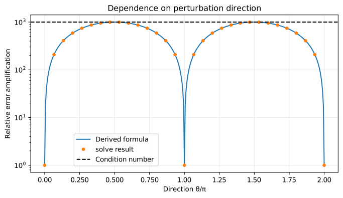
Next, keep the error magnitude fixed and change only its direction. For an error $\Delta\mathbf{b}=\eta(\cos\theta,\sin\theta)^{\mathsf T}$, the solution change is $\eta(\cos\theta,\sin\theta/\alpha)^{\mathsf T}$. The amplification of relative error is
$$ \frac{\|\Delta\mathbf{x}\|_2/\|\mathbf{x}\|_2} {\|\Delta\mathbf{b}\|_2/\|\mathbf{b}\|_2} =\sqrt{\cos^2\theta+\frac{\sin^2\theta}{\alpha^2}}. $$
The factor is one at $\theta=0$ and $1/\alpha$ at $\theta=\pi/2$. Errors of the same size can therefore have different effects depending on their direction.
# Rotate an input error of fixed magnitude and compare amplification factors.
angles = np.linspace(0, 2 * np.pi, 361)
amplifications = []
for angle in angles:
    perturbation = eta * np.array([np.cos(angle), np.sin(angle)])
    perturbed_x = np.linalg.solve(A, b + perturbation)
    relative_change = np.linalg.norm(perturbed_x - x) / np.linalg.norm(x)
    amplifications.append(relative_change / eta)

direction_formula = np.sqrt(np.cos(angles)**2 + np.sin(angles)**2 / alpha**2)
fig, ax = plt.subplots(layout="constrained")
ax.semilogy(angles / np.pi, direction_formula, label="Derived formula")
ax.semilogy(
    angles[::12] / np.pi, np.array(amplifications)[::12],
    "o", markersize=4, label="solve result",
)
ax.axhline(np.linalg.cond(A), color="black", linestyle="--", label="Condition number")
ax.set(xlabel=r"Direction $\theta/\pi$", ylabel="Relative error amplification",
       title="Dependence on perturbation direction")
ax.legend(loc="lower left", bbox_to_anchor=(0.130, 0.0200))
save_figure(fig, "02_direction_and_amplification.svg")
SVG saved to: figures/02_direction_and_amplification.svg
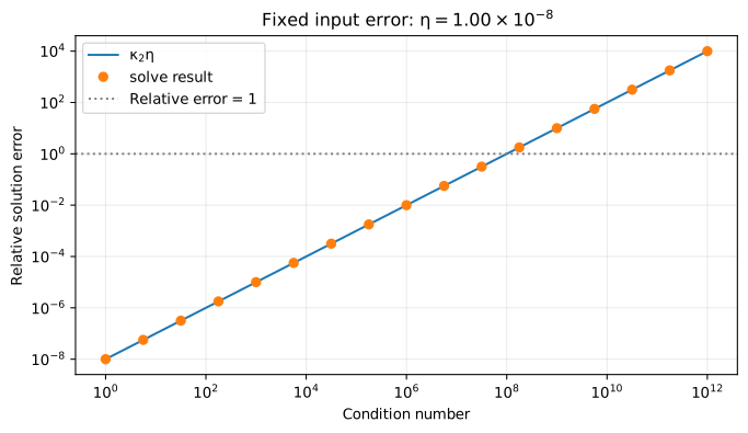
Now fix the relative error in the right-hand side at $\eta=1.00\times10^{-8}$ and perturb it in the direction of greatest amplification. Vary $\alpha$ to increase the condition number and check that the relative solution error grows in proportion to it.
# Fix the input error and test the condition-number relation in the most amplified direction.
eta_sweep = 1.00e-8
alphas = np.logspace(0, -12, 49)
condition_numbers = []
relative_errors = []
for alpha_value in alphas:
    matrix = np.diag([1, alpha_value])
    changed = np.linalg.solve(matrix, b + np.array([0, eta_sweep]))
    condition_numbers.append(np.linalg.cond(matrix))
    relative_errors.append(np.linalg.norm(changed - x) / np.linalg.norm(x))
condition_numbers = np.array(condition_numbers)
relative_errors = np.array(relative_errors)

print("Each row: condition number, relative input error, relative solution error")
pprint(np.column_stack([
    condition_numbers[::16], np.full(4, eta_sweep), relative_errors[::16],
]))
fig, ax = plt.subplots(layout="constrained")
ax.loglog(condition_numbers, condition_numbers * eta_sweep, label=r"$\kappa_2\eta$")
ax.loglog(condition_numbers[::3], relative_errors[::3], "o", label="solve result")
ax.axhline(1, color="gray", linestyle=":", label="Relative error = 1")
ax.set(xlabel="Condition number", ylabel="Relative solution error",
       title="Fixed input error: " + rf"$\eta={latex_number(eta_sweep)}$")
ax.legend()
save_figure(fig, "03_condition_number_and_error.svg")
Each row: condition number, relative input error, relative solution error
array([[1.00e+00, 1.00e-08, 1.00e-08],
       [1.00e+04, 1.00e-08, 1.00e-04],
       [1.00e+08, 1.00e-08, 1.00e+00],
       [1.00e+12, 1.00e-08, 1.00e+04]])


SVG saved to: figures/03_condition_number_and_error.svg
4. The determinant’s size is not enough
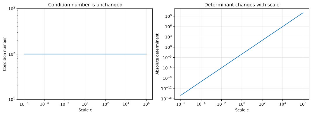
Multiplying an entire matrix $\mathbf{A}$ by a nonzero constant $c$ leaves its condition number unchanged. However, the determinant of a square matrix of size $n$ is multiplied by $c^n$.
$$ \begin{aligned} \kappa_2(c\mathbf{A}) &=\|c\mathbf{A}\|_2\|(c\mathbf{A})^{-1}\|_2\\ &=|c|\|\mathbf{A}\|_2\frac{1}{|c|}\|\mathbf{A}^{-1}\|_2 =\kappa_2(\mathbf{A}),\\ \det(c\mathbf{A})&=c^n\det(\mathbf{A}). \end{aligned} $$
A small absolute determinant alone therefore does not imply strong input-error amplification. The next plot compares the condition number and absolute determinant when scaling the same matrix.
base_matrix = np.diag([1, 0.0100])
scales = np.logspace(-6, 6, 49)
scaled_conditions = np.array([np.linalg.cond(c * base_matrix) for c in scales])
scaled_determinants = np.array([abs(np.linalg.det(c * base_matrix)) for c in scales])

fig, axes = plt.subplots(1, 2, figsize=(11, 4), layout="constrained")
# Set vertical limits before plotting to avoid automatic range selection for a constant series.
axes[0].set(xscale="log", yscale="log", ylim=(10, 1000))
axes[0].plot(scales, scaled_conditions)
axes[0].set(xlabel="Scale c", ylabel="Condition number",
            title="Condition number is unchanged")
axes[1].loglog(scales, scaled_determinants)
axes[1].set(xlabel="Scale c", ylabel="Absolute determinant",
            title="Determinant changes with scale")
save_figure(fig, "04_scaling_and_determinant.svg")
SVG saved to: figures/04_scaling_and_determinant.svg
5. Residuals and algorithm stability
Let $\widehat{\mathbf{x}}$ be an approximate solution and define the residual as $\mathbf{r}=\mathbf{b}-\mathbf{A}\widehat{\mathbf{x}}$.
$$ \begin{aligned} \mathbf{r}&=\mathbf{A}\mathbf{x}-\mathbf{A}\widehat{\mathbf{x}} =\mathbf{A}(\mathbf{x}-\widehat{\mathbf{x}}),\\ \mathbf{x}-\widehat{\mathbf{x}}&=\mathbf{A}^{-1}\mathbf{r},\\ \frac{\|\mathbf{x}-\widehat{\mathbf{x}}\|_2}{\|\mathbf{x}\|_2} &\le\kappa_2(\mathbf{A})\frac{\|\mathbf{r}\|_2}{\|\mathbf{b}\|_2}. \end{aligned} $$
Using the same $\mathbf{A}$ and $\mathbf{b}$ as in Section 3, deliberately choose $\widehat{\mathbf{x}}=(1,1)^{\mathsf T}$ as an approximate solution. The residual is then $\mathbf{r}=(0,-\alpha)^{\mathsf T}$. The relative residual is $\alpha$, but the relative solution error is one. Reducing $\alpha$ makes the relative residual arbitrarily small without changing the relative solution error. A small residual alone therefore cannot guarantee solution accuracy.
# This is a chosen approximation, not solve output, designed to show the difference between residual and error.
x_hat = np.array([1, 1], dtype=float)
relative_residuals = []
forward_errors = []
for alpha_value in alphas:
    matrix = np.diag([1, alpha_value])
    residual = b - matrix @ x_hat
    relative_residuals.append(np.linalg.norm(residual) / np.linalg.norm(b))
    forward_errors.append(np.linalg.norm(x_hat - x) / np.linalg.norm(x))
relative_residuals = np.array(relative_residuals)
forward_errors = np.array(forward_errors)

print("Each row: condition number, relative residual, relative solution error")
pprint(np.column_stack([
    condition_numbers[::16], relative_residuals[::16], forward_errors[::16],
]))
fig, ax = plt.subplots(layout="constrained")
ax.loglog(condition_numbers, relative_residuals, label="Relative residual")
ax.loglog(condition_numbers, forward_errors, label="Relative solution error")
ax.loglog(
    condition_numbers[::3], (condition_numbers * relative_residuals)[::3],
    "o", label="Condition number x relative residual",
)
ax.set(xlabel="Condition number", ylabel="Relative magnitude",
       title="Small residual with an inaccurate solution")
ax.legend()
save_figure(fig, "05_residual_and_solution_error.svg")
Each row: condition number, relative residual, relative solution error
array([[1.00e+00, 1.00e+00, 1.00e+00],
       [1.00e+04, 1.00e-04, 1.00e+00],
       [1.00e+08, 1.00e-08, 1.00e+00],
       [1.00e+12, 1.00e-12, 1.00e+00]])
SVG saved to: figures/05_residual_and_solution_error.svg
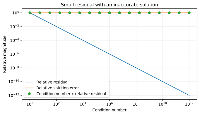
The relation $\mathbf{A}\widehat{\mathbf{x}}=\mathbf{b}-\mathbf{r}$ shows that changing the right-hand side by $-\mathbf{r}$ makes the approximate solution $\widehat{\mathbf{x}}$ an exact solution of the changed system. Thus, the relative residual is the relative backward error when only the right-hand side may change. Forward error measures the difference between the approximation and the exact solution of the original system; here, it is evaluated as relative solution error.
A backward-stable algorithm returns the exact solution of a problem whose inputs differ by small amounts comparable to rounding errors. For a problem with a large condition number, however, a small input change can cause a large solution change. Conditioning is a property of the problem; stability is a property of the algorithm.
If the relative right-hand-side error is $10^{-p}$ and the condition number is $10^q$, the relative solution error is bounded by $10^{q-p}$. When $p>q$, about $q$ significant digits can be lost in the worst case. When $p\le q$, the bound is at least one, so it cannot guarantee any significant digits. The actual number of lost digits depends on the directions of the right-hand side and error. Increasing calculation precision alone cannot remove measurement errors in the input.
Conclusion
For a fixed matrix, the relative solution error caused by a right-hand-side error is at most the condition number times the relative input error. Suitable choices of the right-hand side and error direction can attain this bound.
The 2-norm condition number is the ratio of the largest and smallest singular values. Actual amplification depends on the directions of the right-hand side and error. To assess solution accuracy, check the condition number, input accuracy, and algorithm stability as well as the residual.