Newton法はなぜ2次収束するのか
※ 本記事は2015年に作成した記事のリライトになります。なお、内容は当時のものを基にしていますが、Pythonやライブラリのバージョンは最新のものを使用しています。
実行環境
Python 3.14.6(仮想環境、Jupyter Notebook)。
概要
Newton法は、接線と横軸の交点の$x$座標を次の近似解とする反復法である。関数が2回連続微分可能で、単純根の十分近くから反復を始めると、誤差の1次の項が打ち消され、少なくとも2次で収束する。
本記事では、誤差の関係式をTaylor展開から導き、$x^2-2=0$の正の解を求める計算で確かめる。重根で収束が遅くなる理由や、初期値によって収束しない例、丸め誤差による精度の限界も扱う。
計算の準備
Jupyter Notebookで仮想環境のカーネルを選び、以下のコードを上から順に実行する。使用したライブラリのバージョンとOSは、次の出力に示す。
小数は表示時にのみ有効数字3桁に丸め、計算には丸める前の値を使う。ただし、演算自体には float や Decimal の精度に応じた丸め誤差が生じる。グラフは実行ディレクトリの 101_nb_files にSVG形式で保存し、出力欄にもSVG形式で表示する。
import platform
import sys
from decimal import Decimal, getcontext
from importlib.metadata import version
from pathlib import Path
from pprint import pprint

import matplotlib.pyplot as plt
import numpy as np
import sympy as sp
from IPython.display import Math, display
from matplotlib.ticker import FuncFormatter, MaxNLocator
from matplotlib_inline.backend_inline import set_matplotlib_formats

%matplotlib inline
set_matplotlib_formats("svg")

assert platform.python_version() == "3.14.6"
assert sys.prefix != sys.base_prefix
print("環境名: wa-src(3.14.6)")
print("Python:", platform.python_version())
print("OS:", platform.platform())
print("実行ファイル:", sys.executable)
pprint({name: version(name) for name in ("numpy", "matplotlib", "sympy")})

# 誤差の評価には120桁の十進演算を使う。グラフ用の配列だけfloatに変換する。
getcontext().prec = 120
np.set_printoptions(formatter={"float_kind": lambda value: f"{value:.2e}"})
figure_dir = Path("101_nb_files")
figure_dir.mkdir(exist_ok=True)
plt.rcParams.update({"font.size": 11, "svg.fonttype": "none"})


def tick_label(value, position):
    """整数はそのまま、小数は末尾の0を含む有効数字3桁で表示する。"""
    if float(value).is_integer() and abs(value) < 1000:
        return str(int(value))
    return f"{value:#.3g}"


def save_figure(fig, name):
    """軸の表示を整え、図をSVGファイルに保存し、出力欄にも表示する。"""
    for ax in fig.axes:
        if ax.get_xscale() == "linear":
            ax.xaxis.set_major_formatter(FuncFormatter(tick_label))
        if ax.get_yscale() == "linear":
            ax.yaxis.set_major_formatter(FuncFormatter(tick_label))
        ax.grid(True, alpha=0.250)
    fig.tight_layout()
    fig.savefig(figure_dir / name, format="svg", bbox_inches="tight")
    plt.show()
    plt.close(fig)
環境名: wa-src(3.14.6)
Python: 3.14.6
OS: macOS-26.5.2-arm64-arm-64bit-Mach-O
実行ファイル: /Users/hiroshi/private/wa_src/.venv/bin/python
{'matplotlib': '3.11.2', 'numpy': '2.5.4', 'sympy': '1.14.0'}
1. 接線から更新式を作る
方程式$f(x)=0$の解を$\alpha$、近似解を$x_n$とする。点$(x_n,f(x_n))$における接線を$y=q_n(x)$とおく。$f^{\prime}(x_n)\ne0$なら、接線と横軸の交点の$x$座標は次のように求められる。
$$ \displaystyle \begin{gathered} q_n(x)=f(x_n)+f^{\prime}(x_n)(x-x_n),\\ 0=f(x_n)+f^{\prime}(x_n)(x_{n+1}-x_n),\\ x_{n+1}-x_n=-\frac{f(x_n)}{f^{\prime}(x_n)},\\ x_{n+1}=x_n-\frac{f(x_n)}{f^{\prime}(x_n)}. \end{gathered} $$
以下の関数は、指定した回数を上限にNewton法を反復し、近似解の履歴を返す。関数値が0になった時点で反復を終え、更新時に導関数が0なら例外を発生させる。実際の計算では、反復回数の上限に加え、更新量$|x_{n+1}-x_n|$と残差$|f(x_n)|$に基づく停止判定も必要である。
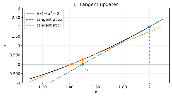
図1には、$f(x)=x^2-2$に対し、$x_0=2$から始めた最初の2回の更新を示す。
def newton_history(f, df, x0, steps):
    """floatとDecimalのどちらでも使える、回数に上限を設けたNewton反復。"""
    x = x0
    values = [x]
    for _ in range(steps):
        fx = f(x)
        if fx == 0:
            break
        slope = df(x)
        if slope == 0:
            raise ZeroDivisionError("導関数が0のため更新できない")
        x = x - fx / slope
        values.append(x)
    return values


def f(x):
    return x**2 - 2


def df(x):
    return 2 * x


xs_float = newton_history(f, df, 2.00, 7)
grid = np.linspace(1.10, 2.10, 400)
fig, ax = plt.subplots(figsize=(7, 4))
ax.plot(grid, f(grid), color="black", label=r"$f(x)=x^2-2$")
ax.axhline(0, color="gray", linewidth=1)
for n, color in enumerate(("tab:blue", "tab:orange")):
    xn, xn_next = xs_float[n:n + 2]
    ax.plot(grid, f(xn) + df(xn) * (grid - xn), "--",
            color=color, label=rf"tangent at $x_{n}$")
    ax.plot([xn, xn], [0, f(xn)], ":", color=color)
    ax.scatter([xn, xn_next], [f(xn), 0], color=color, zorder=3)
    ax.annotate(rf"$x_{n + 1}$", (xn_next, 0), xytext=(5, -18),
                textcoords="offset points", color=color)
ax.set(xlabel="$x$", ylabel="$y$", ylim=(-1, 3), title="1. Tangent updates")
ax.legend()
save_figure(fig, "01_tangents.svg")
2. 誤差の1次の項が消える
$f(\alpha)=0$かつ$f^{\prime}(\alpha)\ne0$を満たす根$\alpha$を単純根という。ここでは、さらに$f$が$\alpha$の近傍で2回連続微分可能であるとする。
誤差を$e_n=x_n-\alpha$とおき、$x_n$を中心とするTaylor展開で$f(\alpha)$を表す。剰余項に現れる$\xi_n$は、$x_n$と$\alpha$の間の点である。
$$ \displaystyle \begin{aligned} 0&=f(\alpha)\\ &=f(x_n)+f^{\prime}(x_n)(\alpha-x_n)\\ &\quad+\frac{f^{\prime\prime}(\xi_n)}{2}(\alpha-x_n)^2\\ &=f(x_n)-f^{\prime}(x_n)e_n+\frac{f^{\prime\prime}(\xi_n)}{2}e_n^2. \end{aligned} $$
両辺を整理し、$f^{\prime}(x_n)$で割ると、
$$ \displaystyle \begin{aligned} f(x_n)&=f^{\prime}(x_n)e_n-\frac{f^{\prime\prime}(\xi_n)}{2}e_n^2,\\ \frac{f(x_n)}{f^{\prime}(x_n)}&=e_n-\frac{f^{\prime\prime}(\xi_n)}{2f^{\prime}(x_n)}e_n^2. \end{aligned} $$
となる。これを更新式に代入する。
$$ \displaystyle \begin{aligned} e_{n+1}&=x_{n+1}-\alpha\\ &=x_n-\alpha-\frac{f(x_n)}{f^{\prime}(x_n)}\\ &=e_n-\left(e_n-\frac{f^{\prime\prime}(\xi_n)}{2f^{\prime}(x_n)}e_n^2\right)\\ &=\frac{f^{\prime\prime}(\xi_n)}{2f^{\prime}(x_n)}e_n^2. \end{aligned} $$
更新式の$e_n$が、$f(x_n)/f^{\prime}(x_n)$に含まれる1次の項と打ち消し合い、$e_n^2$を含む項が残る。この式から2次収束を示すには、反復点が根の近くにとどまり、誤差が0に近づくことも確かめる必要がある。
収束を保証する初期値の条件
$\alpha$を内部に含む十分小さい閉区間$I$を取り、この区間で$|f^{\prime}(x)|\ge m>0$、$|f^{\prime\prime}(x)|\le M$とする。正の定数$K\ge M/(2m)$を取り、$[\alpha-\delta,\alpha+\delta]\subseteq I$かつ$K\delta\le1/2$を満たす$\delta>0$を選ぶ。初期誤差が$|e_0|\le\delta$なら、
$$ \displaystyle |e_{n+1}|\le K|e_n|^2\le\frac12|e_n|\le\delta $$
が帰納的に成り立つ。反復点は区間内にとどまり、$e_n\to0$となる。したがって、収束を初めから仮定する必要はない。
さらに、$f^{\prime\prime}(\alpha)\ne0$で、有限回で解に到達しない場合を考える。このとき、次の極限が正となり、収束次数はちょうど2である。
$$ \displaystyle \lim_{n\to\infty}\frac{|e_{n+1}|}{|e_n|^2} =\left|\frac{f^{\prime\prime}(\alpha)}{2f^{\prime}(\alpha)}\right|=C>0. $$
$f^{\prime\prime}(\alpha)=0$なら、2次より高い次数で収束したり、有限回で解に到達したりすることもある。「少なくとも2次」は誤差が$K|e_n|^2$以下に抑えられることを指し、「ちょうど2次」は上の極限が正の値になることを指す。
3. 平方根の計算で確かめる
$f(x)=x^2-2$、$\alpha=\sqrt2$では、誤差の式を直接整理できる。
$$ \displaystyle \begin{aligned} x_{n+1}&=x_n-\frac{x_n^2-2}{2x_n} =\frac{x_n^2+2}{2x_n},\\ e_{n+1}&=\frac{x_n^2+2-2\alpha x_n}{2x_n}\\ &=\frac{x_n^2+\alpha^2-2\alpha x_n}{2x_n}\\ &=\frac{(x_n-\alpha)^2}{2x_n} =\frac{e_n^2}{2x_n},\\ C&=\frac{1}{2\sqrt2}\approx0.354. \end{aligned} $$
SymPyでもこの恒等式を確認する。数式の出力には display() を使う。
x = sp.symbols("x", positive=True)
alpha_symbol = sp.sqrt(2)
next_error = x - (x**2 - 2) / (2 * x) - alpha_symbol
expected = (x - alpha_symbol)**2 / (2 * x)
assert sp.simplify(next_error - expected) == 0
display(Math(r"x-\frac{x^2-2}{2x}-\sqrt{2}=" + sp.latex(expected)))
display(Math(r"C=\frac{1}{2\sqrt{2}}\approx0.354"))
$$ \displaystyle x-\frac{x^2-2}{2x}-\sqrt{2}=\frac{\left(x - \sqrt{2}\right)^{2}}{2 x} $$
$$ \displaystyle C=\frac{1}{2\sqrt{2}}\approx0.354 $$
高精度計算と通常の浮動小数点計算
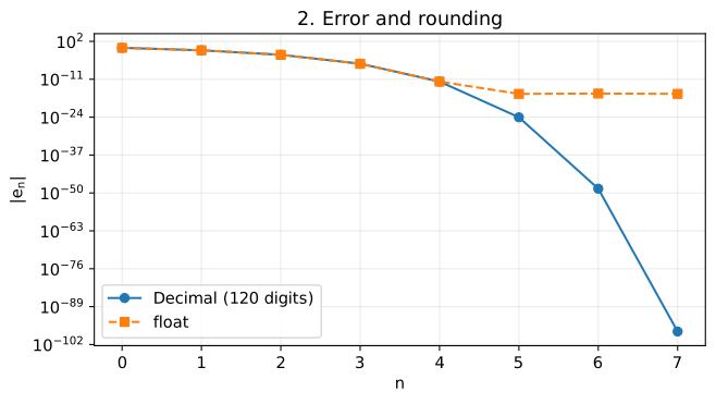
精度を120桁に設定した Decimal で$\sqrt2$と誤差を計算する。float で求めた近似解の誤差も、この基準値との差で評価する。float で表した値どうしの差を取ると、基準値も float に丸められるため、誤差が残っていても差が0になることがある。
図2では高精度計算の誤差が急減する一方、float による計算の誤差は$10^{-16}$程度で停滞する。ここで示した2次収束は、丸め誤差のない演算を仮定した性質である。有限の精度で計算すると、丸め誤差によって誤差の減少が止まる。
alpha = Decimal(2).sqrt()
xs = newton_history(f, df, Decimal(2), 7)
errors = [abs(xn - alpha) for xn in xs]
float_errors = [abs(Decimal.from_float(xn) - alpha) for xn in xs_float]
ratios = [errors[n + 1] / errors[n]**2 for n in range(len(errors) - 1)]

# 小数は指数表記で有効数字3桁にそろえ、結果をリストにまとめてpprintで表示する。
rows = []
for n, (xn, error) in enumerate(zip(xs, errors)):
    rows.append({"n": n, "x_n": f"{xn:.2E}", "abs_error": f"{error:.2E}"})
pprint(rows, sort_dicts=False)

fig, ax = plt.subplots(figsize=(7, 4))
ax.semilogy(range(len(errors)), [float(e) for e in errors], "o-", label="Decimal (120 digits)")
ax.semilogy(range(len(float_errors)), [float(e) for e in float_errors], "s--", label="float")
ax.xaxis.set_major_locator(MaxNLocator(integer=True))
ax.set(xlabel="$n$", ylabel=r"$|e_n|$", title="2. Error and rounding")
ax.legend()
save_figure(fig, "02_errors.svg")
[{'n': 0, 'x_n': '2.00E+0', 'abs_error': '5.86E-1'},
 {'n': 1, 'x_n': '1.50E+0', 'abs_error': '8.58E-2'},
 {'n': 2, 'x_n': '1.42E+0', 'abs_error': '2.45E-3'},
 {'n': 3, 'x_n': '1.41E+0', 'abs_error': '2.12E-6'},
 {'n': 4, 'x_n': '1.41E+0', 'abs_error': '1.59E-12'},
 {'n': 5, 'x_n': '1.41E+0', 'abs_error': '8.99E-25'},
 {'n': 6, 'x_n': '1.41E+0', 'abs_error': '2.86E-49'},
 {'n': 7, 'x_n': '1.41E+0', 'abs_error': '2.89E-98'}]
誤差比と収束次数
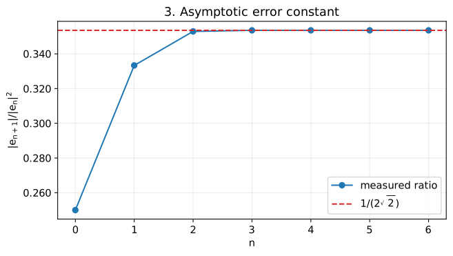
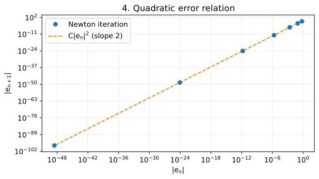
図3では、誤差比$|e_{n+1}|/|e_n|^2$が理論値$C=1/(2\sqrt2)$(約$0.354$)に近づく。図4は、横軸に$|e_n|$、縦軸に$|e_{n+1}|$を取った両対数図である。
$$ \displaystyle \log|e_{n+1}|\approx\log C+2\log|e_n| $$
という関係から、点は傾き2の直線に近づく。さらに、連続する3つの誤差から求めた収束次数の推定値
$$ \displaystyle p_n=\frac{\log(|e_{n+1}|/|e_n|)}{\log(|e_n|/|e_{n-1}|)} $$
も2に近づく。この例では、近似解を有効数字3桁で表示すると同じ値に見えるが、誤差は反復のたびに小さくなっている。
constant = 1 / (2 * alpha)
orders = [
    (errors[n + 1] / errors[n]).ln() / (errors[n] / errors[n - 1]).ln()
    for n in range(1, len(errors) - 1)
]
pprint({"error_ratios": [f"{r:.2E}" for r in ratios],
        "estimated_orders": [f"{p:.2E}" for p in orders]}, sort_dicts=False)

fig, ax = plt.subplots(figsize=(7, 4))
ax.plot(range(len(ratios)), [float(r) for r in ratios], "o-", label="measured ratio")
ax.axhline(float(constant), color="tab:red", linestyle="--", label=r"$1/(2\sqrt{2})$")
ax.xaxis.set_major_locator(MaxNLocator(integer=True))
ax.set(xlabel="$n$", ylabel=r"$|e_{n+1}|/|e_n|^2$", title="3. Asymptotic error constant")
ax.legend()
save_figure(fig, "03_error_ratios.svg")

previous_errors = np.array([float(e) for e in errors[:-1]])
next_errors = np.array([float(e) for e in errors[1:]])
fig, ax = plt.subplots(figsize=(7, 4))
ax.loglog(previous_errors, next_errors, "o", label="Newton iteration", zorder=3)
ax.loglog(previous_errors, float(constant) * previous_errors**2, "--", label=r"$C|e_n|^2$ (slope 2)")
ax.set(xlabel=r"$|e_n|$", ylabel=r"$|e_{n+1}|$", title="4. Quadratic error relation")
ax.legend()
save_figure(fig, "04_error_relation.svg")
{'error_ratios': ['2.50E-1',
                  '3.33E-1',
                  '3.53E-1',
                  '3.54E-1',
                  '3.54E-1',
                  '3.54E-1',
                  '3.54E-1'],
 'estimated_orders': ['1.85E+0',
                      '1.98E+0',
                      '2.00E+0',
                      '2.00E+0',
                      '2.00E+0',
                      '2.00E+0']}
4. 2次収束しない場合
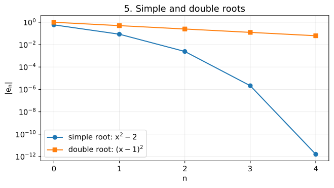
重根では1次収束になる
$f(x)=(x-1)^2$では$f^{\prime}(1)=0$となり、単純根の条件を満たさない。$x_n\ne1$なら、次の関係が成り立つ。
$$ \displaystyle \begin{aligned} x_{n+1}&=x_n-\frac{(x_n-1)^2}{2(x_n-1)} =x_n-\frac{x_n-1}{2},\\ e_{n+1}&=x_n-1-\frac{x_n-1}{2}=\frac12e_n. \end{aligned} $$
誤差は反復のたびに半分になる。より一般に、$m\ge2$を整数とすると、$f(x)=(x-\alpha)^m$では$e_{n+1}=(1-1/m)e_n$となる。図5では、縦軸を対数目盛にすると、重根の誤差を表す点が直線上に並ぶ。これは、反復のたびに誤差が一定の割合で減るためである。
multiple_xs = newton_history(lambda x: (x - 1)**2, lambda x: 2 * (x - 1), Decimal(2), 7)
multiple_errors = [abs(xn - 1) for xn in multiple_xs]
pprint({"multiple_root_ratios": [
    f"{multiple_errors[n + 1] / multiple_errors[n]:.2E}"
    for n in range(len(multiple_errors) - 1)
]})

# 最初の5点を比較し、重根の直線的な減少を読み取りやすくする。
fig, ax = plt.subplots(figsize=(7, 4))
ax.semilogy(range(5), [float(e) for e in errors[:5]], "o-", label=r"simple root: $x^2-2$")
ax.semilogy(range(5), [float(e) for e in multiple_errors[:5]], "s-", label=r"double root: $(x-1)^2$")
ax.xaxis.set_major_locator(MaxNLocator(integer=True))
ax.set(xlabel="$n$", ylabel=r"$|e_n|$", title="5. Simple and double roots")
ax.legend()
save_figure(fig, "05_multiple_root.svg")
{'multiple_root_ratios': ['5.00E-1',
                          '5.00E-1',
                          '5.00E-1',
                          '5.00E-1',
                          '5.00E-1',
                          '5.00E-1',
                          '5.00E-1']}
初期値によっては収束しない
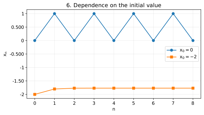
$f(x)=x^3-2x+2$に対して$x_0=0$とすると、
$$ \displaystyle x_1=0-\frac{2}{-2}=1,\qquad x_2=1-\frac{1}{1}=0 $$
となり、反復点は0と1を行き来する。図6では、この反復を、$x_0=-2$から始めて根に収束する反復と比較している。導関数が0でなくても、初期値が根から遠ければ収束は保証されない。
def cubic(x):
    return x**3 - 2 * x + 2


def cubic_derivative(x):
    return 3 * x**2 - 2


cycle = newton_history(cubic, cubic_derivative, Decimal(0), 8)
convergent = newton_history(cubic, cubic_derivative, Decimal(-2), 8)
pprint({"x0=0": [f"{xn:.2E}" if xn != 0 else "0" for xn in cycle],
        "x0=-2, final": f"{convergent[-1]:.2E}"}, sort_dicts=False)

fig, ax = plt.subplots(figsize=(7, 4))
ax.plot(range(len(cycle)), [float(xn) for xn in cycle], "o-", label=r"$x_0=0$")
ax.plot(range(len(convergent)), [float(xn) for xn in convergent], "s-", label=r"$x_0=-2$")
ax.xaxis.set_major_locator(MaxNLocator(integer=True))
ax.set(xlabel="$n$", ylabel="$x_n$", title="6. Dependence on the initial value")
ax.legend()
save_figure(fig, "06_initial_values.svg")
{'x0=0': ['0', '1.00E+0', '0', '1.00E+0', '0', '1.00E+0', '0', '1.00E+0', '0'],
 'x0=-2, final': '-1.77E+0'}
結論
Newton法では、更新式で誤差の1次の項が打ち消される。関数が2回連続微分可能で、単純根の十分近くから反復を始めれば、少なくとも2次で収束する。有限回で解に到達せず、$f^{\prime\prime}(\alpha)\ne0$なら、収束次数はちょうど2となり、漸近誤差定数は$|f^{\prime\prime}(\alpha)/(2f^{\prime}(\alpha))|$である。
平方根の計算では、この誤差定数と収束次数を数値で確かめた。一方、重根では収束が遅くなり、初期値によっては収束しない。また、有限精度の計算では、丸め誤差の影響で誤差の減少が止まることもある。
参考文献:T. A. Driscoll・R. J. Braun, Fundamentals of Numerical Computation, 4.3 Newton’s method (更新式と誤差解析)。Stanford University, Math 114: Newton’s method 3/3 (局所収束の条件)。