Newton法が収束しない例をPythonで作る
※ 本記事は2015年に作成した記事のリライトになります。なお、内容は当時のものを基にしていますが、Pythonやライブラリのバージョンは最新のものを使用しています。
実行環境
Python 3.14.6(仮想環境、Jupyter Notebook)。
概要
Newton法は、接線と横軸の交点の$x$座標を次の近似解として、方程式$f(x)=0$の解を求める反復法である。
本記事では、反復値が2点を往復する例、解から離れ続ける例、導関数が0で更新できない例をPythonで再現する。更新式から収束しない理由を説明し、関数や接線、反復値、残差をグラフで確認する。最後に、初期値を変えた場合とBrent法を使った場合の結果を比較する。
計算の準備
使用したライブラリのバージョンとOSは、次の出力に示す。
以下のコードをJupyter Notebookで上から順に実行すると、グラフが作業ディレクトリの 102_nb_files にSVG形式で保存され、ノートブック内にも表示される。小数は表示時にのみ有効数字3桁に丸め、計算には丸める前の値を使う。
import platform
from pathlib import Path
from pprint import pprint

import matplotlib
import matplotlib.pyplot as plt
import numpy as np
import scipy
from IPython.display import Math, display
from matplotlib.ticker import FuncFormatter, MaxNLocator
from matplotlib_inline.backend_inline import set_matplotlib_formats
from scipy.optimize import brentq, newton

%matplotlib inline
set_matplotlib_formats("svg")

print("実行環境: wa-src(3.14.6)")
print("Python:", platform.python_version())
print("OS:", platform.system(), platform.release())
print("NumPy:", np.__version__)
print("SciPy:", scipy.__version__)
print("Matplotlib:", matplotlib.__version__)

# 配列と目盛りの小数を有効数字3桁で表示する。
np.set_printoptions(formatter={"float_kind": lambda x: f"{x:#.3g}"})
plt.rcParams.update({"font.size": 11, "axes.grid": True, "grid.alpha": 0.250})
output_dir = Path("102_nb_files")
output_dir.mkdir(exist_ok=True)


def save_figure(fig, filename, iteration=False):
    for ax in fig.axes:
        ax.xaxis.set_major_formatter(FuncFormatter(lambda x, pos: f"{x:#.3g}"))
        ax.yaxis.set_major_formatter(FuncFormatter(lambda y, pos: f"{y:#.3g}"))
        if iteration:
            ax.xaxis.set_major_locator(MaxNLocator(integer=True))
            ax.xaxis.set_major_formatter(FuncFormatter(lambda x, pos: f"{x:.0f}"))
    fig.savefig(output_dir / filename, format="svg", bbox_inches="tight")
    plt.show()
    plt.close(fig)
実行環境: wa-src(3.14.6)
Python: 3.14.6
OS: Darwin 25.5.0
NumPy: 2.5.4
SciPy: 1.18.1
Matplotlib: 3.11.2
1. 更新式と計算の準備
点$(x_n,f(x_n))$における接線を$t_n(x)$とすると、$x_n$の近くでは$f(x)$を次のように近似できる。
$$ \displaystyle t_n(x)=f(x_n)+f^{\prime}(x_n)(x-x_n)\approx f(x) $$
接線と横軸との交点の$x$座標を、次の近似値$x_{n+1}$とする。$f^{\prime}(x_n)\ne0$なら、次のように変形できる。
$$ \displaystyle \begin{gathered} 0=f(x_n)+f^{\prime}(x_n)(x_{n+1}-x_n),\\ x_{n+1}-x_n=-\frac{f(x_n)}{f^{\prime}(x_n)},\\ x_{n+1}=x_n-\frac{f(x_n)}{f^{\prime}(x_n)}. \end{gathered} $$
$f$が解$r$の近傍で2回連続微分可能で、$f^{\prime}(r)\ne0$なら、$r$に十分近い初期値からは少なくとも2次収束する。ただし、どの初期値からでも収束するわけではない。
以下の関数 newton_trace は、初期値と各反復値を保存し、残差$|f(x_n)|$が$1.00\times10^{-10}$以下になったら反復を終了する。導関数が0になった場合や反復回数の上限に達した場合にも、終了理由を返す。残差の許容値は、この例の計算に合わせて設定したものである。別の問題では、関数値の大きさや必要な精度に応じて調整する。
def newton_trace(f, df, x0, maxiter=12, ftol=1.00e-10):
    """初期値を含む履歴と終了理由を返す。"""
    x = float(x0)
    history = [x]
    for n in range(maxiter + 1):
        fx = float(f(x))
        if not np.isfinite(fx):
            reason = "関数値が有限でない"
            break
        if abs(fx) <= ftol:
            reason = "残差が許容値以下"
            break
        if n == maxiter:
            reason = "反復上限"
            break
        dfx = float(df(x))
        if not np.isfinite(dfx) or dfx == 0:
            reason = "導関数が0または有限でない"
            break
        # 残差を確認してから割るので、解での不要な除算を避けられる。
        x_next = x - fx / dfx
        if not np.isfinite(x_next):
            reason = "更新値が有限でない"
            break
        history.append(x_next)
        x = x_next
    return np.array(history), reason


display(Math(r"x_{n+1}=x_n-\frac{f(x_n)}{f'(x_n)}"))
$$ \displaystyle x_{n+1}=x_n-\frac{f(x_n)}{f^{\prime}(x_n)} $$
2. 0と1を往復する例
$f(x)=x^3-2x+2$、$f^{\prime}(x)=3x^2-2$とし、$x_0=0$から始める。
$$ \displaystyle \begin{aligned} f(0)&=2,\qquad f^{\prime}(0)=-2,\\ x_1&=0-\frac{2}{-2}=1,\\ f(1)&=1-2+2=1,\\ f^{\prime}(1)&=3-2=1,\\ x_2&=1-\frac{1}{1}=0. \end{aligned} $$
2回の更新で初期値に戻るため、$k=0,1,2,\ldots$に対して$x_{2k}=0$、$x_{2k+1}=1$が成り立つ。どちらも解ではなく、残差は2と1を交互に取る。これは丸め誤差ではなく、厳密な計算でも生じる周期2の反復である。
def f_cycle(x):
    return x**3 - 2 * x + 2


def df_cycle(x):
    return 3 * x**2 - 2


cycle, cycle_reason = newton_trace(f_cycle, df_cycle, 0)
print(cycle_reason)
pprint(cycle)
pprint(np.abs(f_cycle(cycle)))

# 2本の接線の横軸との交点が、次の反復値になる。
grid = np.linspace(-2, 2, 401)
fig, ax = plt.subplots(figsize=(8, 5), layout="constrained")
ax.plot(grid, f_cycle(grid), label=r"$f(x)=x^3-2x+2$")
ax.plot(grid, 2 - 2 * grid, "--", label=r"$t_0(x)=2-2x$")
ax.plot(grid, grid, "--", label=r"$t_1(x)=x$")
ax.axhline(0, color="black", linewidth=1)
ax.scatter([0, 1], [2, 1], color="black", zorder=5)
ax.scatter([1, 0], [0, 0], color="tab:red", zorder=5)
ax.set(xlabel="$x$", ylabel="$y$", title="Two-cycle: tangent intersections")
ax.legend()
save_figure(fig, "01_cycle_tangents.svg")

fig, axes = plt.subplots(1, 2, figsize=(10, 4), layout="constrained")
steps = np.arange(cycle.size)
axes[0].plot(steps, cycle, "o-")
axes[0].set(xlabel="$n$", ylabel="$x_n$", title="Iterates: 0, 1, 0, 1, ...")
axes[1].plot(steps, np.abs(f_cycle(cycle)), "o-", color="tab:orange")
axes[1].set(xlabel="$n$", ylabel=r"$|f(x_n)|$", title="Residual: 2, 1, 2, 1, ...")
save_figure(fig, "02_cycle_history.svg", iteration=True)
反復上限
array([0.00, 1.00, 0.00, 1.00, 0.00, 1.00, 0.00, 1.00, 0.00, 1.00, 0.00,
       1.00, 0.00])
array([2.00, 1.00, 2.00, 1.00, 2.00, 1.00, 2.00, 1.00, 2.00, 1.00, 2.00,
       1.00, 2.00])
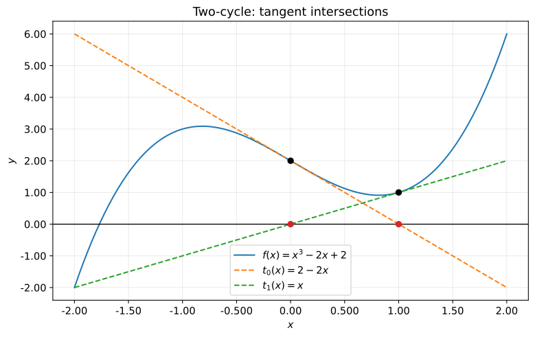
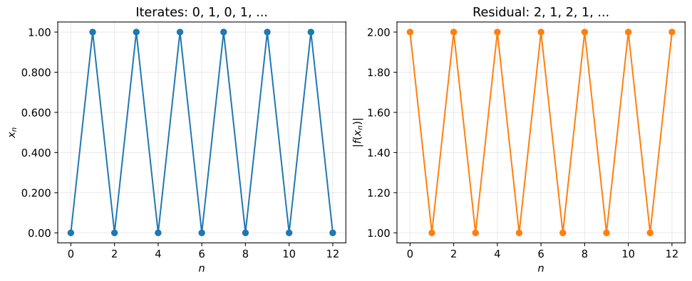
接線は毎回引けるが、反復値は0と1を往復し、残差は0に近づかない。最終値だけでなく数回分の反復値を並べると、この往復を確認できる。
3. 絶対値が2倍ずつ増える例
次に、実数の立方根を返す関数$f(x)=\sqrt[3]{x}$を考える。解は$r=0$である。$y=\sqrt[3]{x}$とすると$x=y^3$なので、$x\ne0$では次のようになる。
$$ \displaystyle \begin{aligned} \frac{dx}{dy}&=3y^2,\\ f^{\prime}(x)&=\frac{dy}{dx}=\frac{1}{3y^2} =\frac{1}{3(\sqrt[3]{x})^2}. \end{aligned} $$
$x_n\ne0$として、これを更新式に代入する。
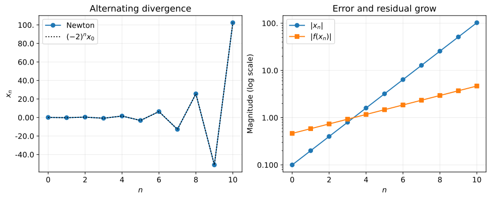
$$ \displaystyle \begin{aligned} x_{n+1} &=x_n-\frac{\sqrt[3]{x_n}}{\frac{1}{3(\sqrt[3]{x_n})^2}}\\ &=x_n-3(\sqrt[3]{x_n})^3\\ &=x_n-3x_n=-2x_n,\\ x_n&=(-2)^n x_0,\qquad |x_n|=2^n|x_0|. \end{aligned} $$
$x_0\ne0$なら、反復値は符号を交互に変えながら解から離れる。残差$|f(x_n)|=2^{n/3}|x_0|^{1/3}$も増え続ける。解$r=0$では$f$は微分できないため、第1節で示した局所収束の条件を満たさない。負の数の立方根も実数として計算するため、実装には np.cbrt を使う。
def f_diverge(x):
    return np.cbrt(x)


def df_diverge(x):
    return 1 / (3 * np.cbrt(x)**2)


diverging, diverging_reason = newton_trace(f_diverge, df_diverge, 0.100, maxiter=10)
print(diverging_reason)
pprint(diverging)

steps = np.arange(diverging.size)
theory = 0.100 * (-2)**steps
fig, axes = plt.subplots(1, 2, figsize=(10, 4), layout="constrained")
axes[0].plot(steps, diverging, "o-", label="Newton")
axes[0].plot(steps, theory, ":", color="black", label=r"$(-2)^n x_0$")
axes[0].set(xlabel="$n$", ylabel="$x_n$", title="Alternating divergence")
axes[0].legend()
axes[1].semilogy(steps, np.abs(diverging), "o-", label=r"$|x_n|$")
axes[1].semilogy(steps, np.abs(f_diverge(diverging)), "s-", label=r"$|f(x_n)|$")
axes[1].set(xlabel="$n$", ylabel="Magnitude (log scale)", title="Error and residual grow")
axes[1].legend()
save_figure(fig, "03_divergence.svg", iteration=True)
反復上限
array([0.100, -0.200, 0.400, -0.800, 1.60, -3.20, 6.40, -12.8, 25.6,
       -51.2, 102.])
4. 導関数が0で更新できない例
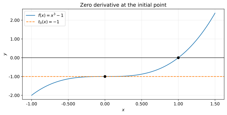
$f(x)=x^3-1$には解$r=1$があるが、初期値を$x_0=0$にすると
$$ \displaystyle f(0)=-1,\qquad f^{\prime}(0)=3\cdot0^2=0 $$
となる。更新式の分母が0になるため、次の近似値$x_1$を計算できない。接線は$y=-1$で、横軸と交わらない。
ここで用いる newton_trace は、0で除算する前に反復を終了し、その理由を返す。なお、導関数が0でも$f(x_n)=0$ならすでに解に到達している。その場合に不要な除算をしないよう、コードでは導関数より先に残差を確認している。
def f_flat(x):
    return x**3 - 1


def df_flat(x):
    return 3 * x**2


stopped, stopped_reason = newton_trace(f_flat, df_flat, 0)
print(stopped_reason)
pprint(stopped)

grid = np.linspace(-1, 1.50, 301)
fig, ax = plt.subplots(figsize=(8, 4), layout="constrained")
ax.plot(grid, f_flat(grid), label=r"$f(x)=x^3-1$")
ax.axhline(-1, linestyle="--", color="tab:orange", label=r"$t_0(x)=-1$")
ax.axhline(0, color="black", linewidth=1)
ax.scatter([0, 1], [-1, 0], color="black", zorder=5)
ax.set(xlabel="$x$", ylabel="$y$", title="Zero derivative at the initial point")
ax.legend()
save_figure(fig, "04_zero_derivative.svg")
導関数が0または有限でない
array([0.00])
5. 初期値と解法を変えて比較する
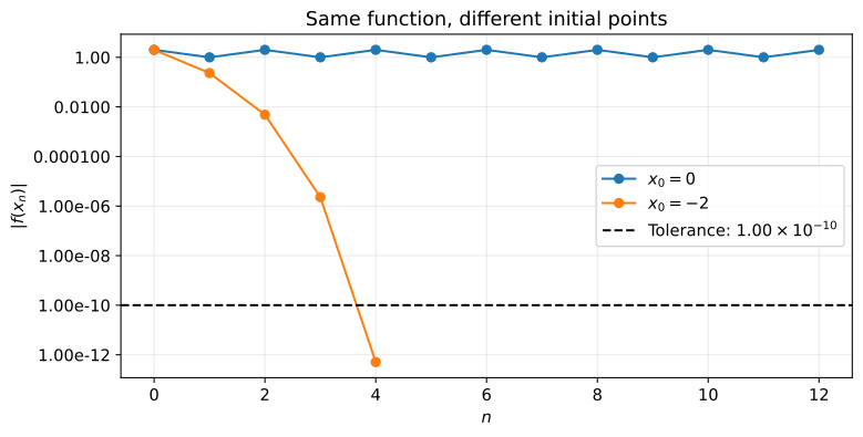
第2節の$f(x)=x^3-2x+2$でも、初期値を$x_0=-2$に変えると収束する。一方、$x_0=0$のまま反復回数の上限を増やしても、0と1の往復は解消しない。
SciPyの newton でNewton法を使うには、導関数を fprime 引数に渡す。fprime を省略すると割線法になる。ここでは disp=False と full_output=True を指定し、収束しなかった場合も最終値と収束状況を受け取れるようにする。
残差を停止判定に使う newton_trace とは異なり、SciPyの newton は更新量$|x_{n+1}-x_n|$を基準に停止を判定する。SciPyの公式ドキュメント
でも結果の検証が必要とされているため、ここでは収束状況と併せて残差も確認する。
また、この多項式は連続であり、区間の両端で
$$ \displaystyle \begin{aligned} f(-2)&=-8+4+2=-2<0,\\ f(-1)&=-1+2+2=3>0. \end{aligned} $$
と符号が異なるため、区間$[-2,-1]$には少なくとも1つの解がある。関数が連続な区間で、両端の関数値の符号が異なる場合は、Brent法 も使える。解は有効数字3桁で表示するが、残差は丸める前の値で計算する。
converging, converging_reason = newton_trace(f_cycle, df_cycle, -2)
print(converging_reason)

# 未収束の戻り値を解と扱わず、収束フラグと残差を並べる。
failed_x, failed_info = newton(
    f_cycle, 0, fprime=df_cycle, maxiter=12, full_output=True, disp=False
)
brent_x, brent_info = brentq(f_cycle, -2, -1, full_output=True)
pprint({
    "Newton x0=0": {
        "converged": failed_info.converged,
        "last_x": f"{failed_x:#.3g}",
        "residual": f"{abs(f_cycle(failed_x)):#.3g}",
    },
    "Newton x0=-2": {
        "last_x": f"{converging[-1]:#.3g}",
        "residual": f"{abs(f_cycle(converging[-1])):#.3g}",
    },
    "Brent [-2, -1]": {
        "converged": brent_info.converged,
        "root": f"{brent_x:#.3g}",
        "residual": f"{abs(f_cycle(brent_x)):#.3g}",
    },
}, sort_dicts=False)
display(Math(r"\hat{x}_{\mathrm{Brent}}\approx " + f"{brent_x:#.3g}"))

fig, ax = plt.subplots(figsize=(8, 4), layout="constrained")
for values, label in [(cycle, "$x_0=0$"), (converging, "$x_0=-2$")]:
    ax.semilogy(np.arange(values.size), np.abs(f_cycle(values)), "o-", label=label)
ax.axhline(1.00e-10, linestyle="--", color="black", label=r"Tolerance: $1.00\times10^{-10}$")
ax.set(xlabel="$n$", ylabel=r"$|f(x_n)|$", title="Same function, different initial points")
ax.legend()
save_figure(fig, "05_initial_values.svg", iteration=True)
残差が許容値以下
{'Newton x0=0': {'converged': False, 'last_x': '0.00', 'residual': '2.00'},
 'Newton x0=-2': {'last_x': '-1.77', 'residual': '5.05e-13'},
 'Brent [-2, -1]': {'converged': True, 'root': '-1.77', 'residual': '1.33e-15'}}
$$ \displaystyle \hat{x}_{\mathrm{Brent}}\approx -1.77 $$
結論
この記事では、Newton法が収束しない3つの例を、更新式とPythonで計算した反復履歴から確認した。
0と1を往復する例では残差が0に近づかず、立方根の例では反復値が解から離れ続けた。導関数が0の例では、更新式の分母が0になり、次の近似値を計算できなかった。
計算結果を解として使う前に、最終値だけでなく、残差、導関数、終了理由を確認する必要がある。初期値を変えると収束する場合もある。また、関数が連続な区間の両端で関数値の符号が異なれば、Brent法も使える。