Hilbert行列はなぜコンピュータにとって難しいのか
※ 本記事は2015年に作成した記事のリライトになります。なお、内容は当時のものを基にしていますが、Pythonやライブラリのバージョンは最新のものを使用しています。
実行環境
Python 3.14.6(仮想環境、Jupyter Notebook)。
概要
Hilbert行列には逆行列が存在する。しかし、この行列を係数行列とする連立一次方程式では、入力のわずかな誤差が解を大きく変えることがある。
本記事では、まずHilbert行列の正則性を示し、条件数を使って誤差が増幅される理由を説明する。そのうえで、Pythonを使い、残差と解の誤差の違い、右辺の変化が解に与える影響、計算精度による違いを確認する。
計算の準備
倍精度計算にはNumPyとSciPy、多倍長計算にはmpmathを使い、グラフはMatplotlibで描画する。使用したライブラリのバージョンは、次の出力に示す。
倍精度の計算結果は実行環境に依存する。条件数が大きい場合には、末尾の桁だけでなく、上位の桁まで異なることがある。
以降のコードは、Jupyter Notebookのセルとして上から順に実行する。小数は表示するときだけ有効数字3桁に丸める。グラフの軸名は英語とし、SVG形式でノートブックに埋め込む。SVGファイルは、実行時の作業ディレクトリにある figures ディレクトリに保存する。
import sys
from pathlib import Path
from pprint import pprint

import matplotlib
import matplotlib.pyplot as plt
import mpmath as mp
import numpy as np
import scipy
from IPython.display import Math, display
from matplotlib.ticker import FuncFormatter, MaxNLocator
from matplotlib_inline.backend_inline import set_matplotlib_formats
from scipy.linalg import hilbert

%matplotlib inline

# 指定したPythonの仮想環境で実行していることを確認する。
assert sys.version_info[:3] == (3, 14, 6)
assert sys.prefix != sys.base_prefix
print(f"実行環境: wa-src({sys.version.split()[0]})")
print(f"NumPy {np.__version__}, SciPy {scipy.__version__}")
print(f"Matplotlib {matplotlib.__version__}, mpmath {mp.__version__}")

# 数値は表示するときだけ有効数字3桁に整える。
# .2eは小数点以下2桁の指数表記であり、有効数字は3桁となる。
np.set_printoptions(formatter={"float_kind": lambda value: f"{value:.2e}"})
tick_formatter = FuncFormatter(lambda value, position: f"{value:#.3g}")

# SVG形式でノートブックに図を埋め込む。
set_matplotlib_formats("svg")
plt.rcParams.update({
    "figure.figsize": (11, 4),
    "figure.dpi": 130,
    "savefig.format": "svg",
    "font.size": 10,
    "axes.grid": True,
    "grid.alpha": 0.250,
})


# 実行時の作業ディレクトリに、SVGの保存先を作る。
figure_dir = Path("figures")
figure_dir.mkdir(parents=True, exist_ok=True)


def scientific_latex(value):
    """数値を有効数字3桁のLaTeX表記に変換する。"""
    mantissa, exponent = f"{float(value):.2e}".split("e")
    return rf"{mantissa}\times 10^{{{int(exponent)}}}"


def make_mp_hilbert(size):
    """現在のmpmathの精度でHilbert行列を生成する。"""
    # 整数をmpmathの数に変換してから割り、倍精度の丸めを避ける。
    # Pythonの添字は0から始まるため、分母はi + j + 1となる。
    return mp.matrix([
        [mp.mpf(1) / (i + j + 1) for j in range(size)]
        for i in range(size)
    ])
実行環境: wa-src(3.14.6)
NumPy 2.5.4, SciPy 1.18.1
Matplotlib 3.11.2, mpmath 1.3.0
1. Hilbert行列の定義と正則性
数式と考え方
添字を1から数えると、$n$ 次のHilbert行列 $\mathbf{H}_n$ は次のように定義される。Pythonの添字は0から始まるため、実装では分母が i + j + 1 となる。SciPyの公式ドキュメント
にも同じ定義がある。
$$ \begin{aligned} \mathbf{H}_n&=(h_{ij}),\qquad h_{ij}=\frac{1}{i+j-1},\\ &\quad 1\le i,j\le n. \end{aligned} $$
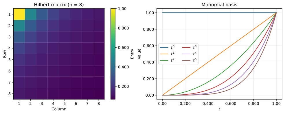
各成分は、単項式どうしの積を区間 $[0,1]$ で積分した値としても表せる。
$$ \begin{aligned} \int_0^1 t^{i-1}t^{j-1}\,dt &=\int_0^1 t^{i+j-2}\,dt\\ &=\left[\frac{t^{i+j-1}}{i+j-1}\right]_0^1\\ &=\frac{1}{i+j-1}. \end{aligned} $$
任意の実ベクトル $\mathbf{c}\ne\mathbf{0}$ に対して、和と積分を入れ替えると次の式が得られる。
$$ \begin{aligned} \mathbf{c}^{\mathsf T}\mathbf{H}_n\mathbf{c} &=\sum_{i=1}^n\sum_{j=1}^n c_i c_j h_{ij}\\ &=\int_0^1\sum_{i=1}^n\sum_{j=1}^n c_i c_j t^{i-1}t^{j-1}\,dt\\ &=\int_0^1\left(\sum_{i=1}^n c_i t^{i-1}\right)^2dt>0. \end{aligned} $$
$\mathbf{c}\ne\mathbf{0}$ なら、この多項式は恒等的に0にはならないため、その二乗の積分は正である。したがって、$\mathbf{H}_n$ は対称正定値行列であり、正則である。
一方、単項式の線形結合では項どうしが相殺し、係数ベクトルのユークリッドノルムが1でも、二乗の積分値が小さくなることがある。この積分値は $\mathbf{c}^{\mathsf T}\mathbf{H}_n\mathbf{c}$ に等しく、ユークリッドノルムが1のベクトル全体での最小値が、$\mathbf{H}_n$ の最小固有値である。したがって、積分値が小さくなる単位ベクトルがあれば、最小固有値も小さいことが分かる。
Pythonによる計算例
# 3次の行列を小数と分数の両方で確認する。
H3 = hilbert(3)
print("Hilbert行列(n = 3、小数表示)")
pprint(H3)

# 数式は文字列としてprintせず、LaTeXとして表示する。
display(
    Math(
        r"\mathbf{H}_3=\begin{bmatrix}"
        r"1 & \frac{1}{2} & \frac{1}{3}\\"
        r"\frac{1}{2} & \frac{1}{3} & \frac{1}{4}\\"
        r"\frac{1}{3} & \frac{1}{4} & \frac{1}{5}"
        r"\end{bmatrix}"
    )
)
Hilbert行列(n = 3、小数表示)
array([[1.00e+00, 5.00e-01, 3.33e-01],
       [5.00e-01, 3.33e-01, 2.50e-01],
       [3.33e-01, 2.50e-01, 2.00e-01]])
$$ \displaystyle \mathbf{H}_3=\begin{bmatrix}1 & \frac{1}{2} & \frac{1}{3}\\\frac{1}{2} & \frac{1}{3} & \frac{1}{4}\\\frac{1}{3} & \frac{1}{4} & \frac{1}{5}\end{bmatrix} $$
fig, axes = plt.subplots(1, 2, layout="constrained")

# 左図: 成分の値を色で表す。行・列番号は数式と同じ1始まりにする。
# 各成分を四角形で描き、SVG内でもベクトル形式を保つ。
cell_edges = np.arange(9) + 0.500
heatmap = axes[0].pcolormesh(
    cell_edges,
    cell_edges,
    hilbert(8),
    cmap="viridis",
    shading="flat",
    edgecolors="face",
    linewidth=0.100,
)
axes[0].set_aspect("equal")
axes[0].invert_yaxis()
axes[0].grid(False)
axes[0].set(title="Hilbert matrix (n = 8)", xlabel="Column", ylabel="Row")
axes[0].set_xticks(range(1, 9))
axes[0].set_yticks(range(1, 9))
colorbar = fig.colorbar(heatmap, ax=axes[0], format=tick_formatter, label="Entry")
# カラーバーもベクトルとして保存する。
colorbar.solids.set_rasterized(False)
# SVG表示時の色の区切りに、白い継ぎ目が出ることを防ぐ。
colorbar.solids.set_edgecolor("face")

# 右図: 行列の成分を積分で表したときに現れる単項式を描く。
t = np.linspace(0, 1, 300)
for degree in range(6):
    axes[1].plot(t, t**degree, label=rf"$t^{degree}$")

axes[1].set(title="Monomial basis", xlabel="t", ylabel="Value")
axes[1].xaxis.set_major_formatter(tick_formatter)
axes[1].yaxis.set_major_formatter(tick_formatter)
axes[1].legend(ncol=2)
# SVGファイルとして保存し、ノートブックにも表示する。
svg_path = figure_dir / "01_hilbert_and_monomials.svg"
fig.savefig(svg_path, format="svg", bbox_inches="tight")
print(f"SVG保存先: {svg_path.as_posix()}")
plt.show()
SVG保存先: figures/01_hilbert_and_monomials.svg
2. 条件数と誤差の増幅
数式と考え方
以下では $\mathbf{H}=\mathbf{H}_n$ と略記し、ベクトルのユークリッドノルムと、それに対応する行列の2ノルムを使う。最大特異値を $\sigma_{\max}$、最小特異値を $\sigma_{\min}$ とすると、条件数は
$$ \kappa_2(\mathbf{H})=\|\mathbf{H}\|_2\|\mathbf{H}^{-1}\|_2 =\frac{\sigma_{\max}}{\sigma_{\min}} $$
である。ここでは $\mathbf{b}\ne\mathbf{0}$ とし、行列 $\mathbf{H}$ を固定して右辺だけを変化させる。
$$ \begin{aligned} \mathbf{H}\mathbf{x}&=\mathbf{b},\\ \mathbf{H}(\mathbf{x}+\Delta\mathbf{x})&=\mathbf{b}+\Delta\mathbf{b},\\ \mathbf{H}\Delta\mathbf{x}&=\Delta\mathbf{b},\\ \Delta\mathbf{x}&=\mathbf{H}^{-1}\Delta\mathbf{b}. \end{aligned} $$
ここで $\|\Delta\mathbf{x}\|_2\le\|\mathbf{H}^{-1}\|_2\|\Delta\mathbf{b}\|_2$、かつ $\|\mathbf{b}\|_2\le\|\mathbf{H}\|_2\|\mathbf{x}\|_2$ である。両者を使うと、次の不等式が得られる。
$$ \begin{aligned} \frac{\|\Delta\mathbf{x}\|_2}{\|\mathbf{x}\|_2} &\le\|\mathbf{H}^{-1}\|_2\|\Delta\mathbf{b}\|_2 \frac{\|\mathbf{H}\|_2}{\|\mathbf{b}\|_2} \\ &=\kappa_2(\mathbf{H})\frac{\|\Delta\mathbf{b}\|_2}{\|\mathbf{b}\|_2}. \end{aligned} $$
この不等式は、右辺の相対誤差に対する解の相対誤差の増幅率が、条件数を超えないことを示す。実際の増幅率は、元の右辺と加えた誤差の方向によって変わる。
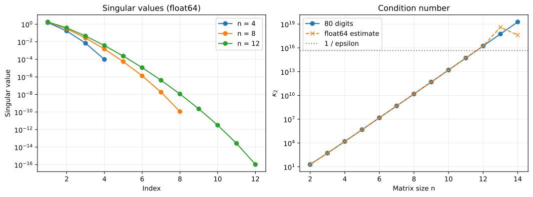
次のコードでは、倍精度の特異値分解で求めた条件数と、十進80桁の多倍長計算で求めた条件数を比較する。対称正定値行列では固有値と特異値が一致するため、多倍長計算では最大・最小固有値の比を使う。
Pythonによる計算例
matrix_sizes = np.arange(2, 15)
condition_float64 = []
condition_high_precision = []

for size in matrix_sizes:
    size = int(size)

    # 倍精度側は特異値分解を使って2ノルムの条件数を求める。
    condition_float64.append(np.linalg.cond(hilbert(size), 2))

    # 対称正定値行列では最大・最小固有値の比も条件数となる。
    with mp.workdps(80):
        eigenvalues = mp.eigsy(make_mp_hilbert(size), eigvals_only=True)
        condition = eigenvalues[size - 1] / eigenvalues[0]

        # 条件数の計算を終えてから、表示・描画用にfloatへ変換する。
        condition_high_precision.append(float(condition))

condition_float64 = np.array(condition_float64)
condition_high_precision = np.array(condition_high_precision)

# 代表的な次数だけを出力し、数値の変化を読み取りやすくする。
condition_summary = []
for size, value64, value80 in zip(matrix_sizes, condition_float64, condition_high_precision):
    if size in (6, 10, 12, 14):
        condition_summary.append(
            {
                "n": int(size),
                "cond_float64": f"{value64:.2e}",
                "cond_80digits": f"{value80:.2e}",
            }
        )

print("次数ごとの条件数(倍精度と80桁計算)")
pprint(condition_summary, sort_dicts=False)
次数ごとの条件数(倍精度と80桁計算)
[{'n': 6, 'cond_float64': '1.50e+07', 'cond_80digits': '1.50e+07'},
 {'n': 10, 'cond_float64': '1.60e+13', 'cond_80digits': '1.60e+13'},
 {'n': 12, 'cond_float64': '1.72e+16', 'cond_80digits': '1.71e+16'},
 {'n': 14, 'cond_float64': '4.05e+17', 'cond_80digits': '1.85e+19'}]
fig, axes = plt.subplots(1, 2, layout="constrained")

# 左図: 小さな特異値まで比較できるように縦軸を対数にする。
for size in (4, 8, 12):
    singular_values = np.linalg.svd(hilbert(size), compute_uv=False)
    indices = np.arange(1, size + 1)
    axes[0].semilogy(indices, singular_values, "o-", label=f"n = {size}")

axes[0].set(
    title="Singular values (float64)",
    xlabel="Index",
    ylabel="Singular value",
)
axes[0].xaxis.set_major_locator(MaxNLocator(integer=True))
axes[0].legend()

# 右図: 同じ次数について、倍精度と多倍長の条件数を比較する。
axes[1].semilogy(matrix_sizes, condition_high_precision, "o-", label="80 digits")
axes[1].semilogy(matrix_sizes, condition_float64, "x--", label="float64 estimate")
axes[1].axhline(
    1 / np.finfo(float).eps,
    color="gray",
    linestyle=":",
    label="1 / epsilon",
)
axes[1].set(title="Condition number", xlabel="Matrix size n", ylabel=r"$\kappa_2$")
axes[1].xaxis.set_major_locator(MaxNLocator(integer=True))
axes[1].legend()
# SVGファイルとして保存し、ノートブックにも表示する。
svg_path = figure_dir / "02_singular_values_and_condition.svg"
fig.savefig(svg_path, format="svg", bbox_inches="tight")
print(f"SVG保存先: {svg_path.as_posix()}")
plt.show()
SVG保存先: figures/02_singular_values_and_condition.svg
計算結果
$n=14$ の条件数は80桁計算で約 $1.85\times10^{19}$ である。本環境の倍精度計算では約 $4.05\times10^{17}$ となり、条件数自体の評価にも誤差が見られる。
3. 丸め誤差と小さな残差
数式と考え方
float64 で表せる数のうち、1と、その次に大きい数との差は $\varepsilon=2^{-52}\approx2.22\times10^{-16}$ である。最近接丸めの単位丸め誤差は $u=\varepsilon/2$ となる。$1/3$ などは有限桁の二進数では正確に表せないため、格納した時点で丸め誤差が入る。Highamの解説
でも、この入力誤差と、誤差が増幅されやすい性質(悪条件性)が指摘されている。
80桁で求めた $\kappa_2(\mathbf{H}_{12})$ は約 $1.71\times10^{16}$ である。この大きさでは、倍精度の丸め誤差が増幅され、解の有効桁が失われることがある。さらに次数が大きくなると、倍精度で求めた条件数自体にも大きな誤差が生じる。
基準となる解を $\mathbf{x}_*=\mathbf{1}$ とし、$\mathbf{b}=\mathbf{H}\mathbf{x}_*$ を計算して連立一次方程式を解く。ここで $\mathbf{1}$ は、全成分が1のベクトルである。ただし、コード中では行列を格納するときと、行列とベクトルの積で右辺を作るときに丸め誤差が入る。得られた数値解を $\widehat{\mathbf{x}}$ とし、基準解に対する相対前進誤差 $E$ と相対残差 $R$ を次のように定義する。
$$ E=\frac{\|\widehat{\mathbf{x}}-\mathbf{x}_*\|_2}{\|\mathbf{x}_*\|_2}, \qquad R=\frac{\|\mathbf{b}-\mathbf{H}\widehat{\mathbf{x}}\|_2}{\|\mathbf{b}\|_2}. $$
ある入力 $\mathbf{H},\mathbf{b}$ に対する厳密な解を $\mathbf{x}$、残差を $\mathbf{r}=\mathbf{b}-\mathbf{H}\widehat{\mathbf{x}}$ とすると、
$$ \mathbf{r}=\mathbf{H}(\mathbf{x}-\widehat{\mathbf{x}}),\qquad \widehat{\mathbf{x}}-\mathbf{x}=-\mathbf{H}^{-1}\mathbf{r}. $$
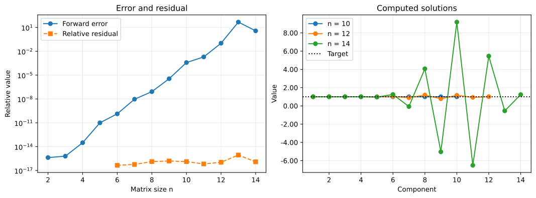
前節と同じ評価により、厳密な解 $\mathbf{x}$ に対する相対前進誤差は $\kappa_2(\mathbf{H})R$ 以下となる。条件数が大きければ、この上限は残差が小さくても大きくなり得るため、残差だけでは解の正確さを判断できない。
この評価の基準となるのは、同じ入力に対する厳密な解 $\mathbf{x}$ である。一方、実験で求める $E$ は $\mathbf{x}_*$ を基準とするため、入力の丸めによるずれも含む。また、実験では残差も倍精度で計算するため、その値自体に丸め誤差が含まれる。対数軸では、計算上0となった残差を表示しない。
Pythonによる計算例
forward_errors = []
relative_residuals = []
computed_solutions = {}

for size in matrix_sizes:
    size = int(size)
    H = hilbert(size)

    # 目標の解を全成分1とし、それに対応する右辺を作る。
    # この行列積にも倍精度の丸めが入る。
    x_true = np.ones(size)
    b = H @ x_true
    x_hat = np.linalg.solve(H, b)

    # 解そのものの誤差と、方程式を満たす程度を別々に評価する。
    forward_error = np.linalg.norm(x_hat - x_true) / np.linalg.norm(x_true)
    relative_residual = np.linalg.norm(b - H @ x_hat) / np.linalg.norm(b)

    forward_errors.append(forward_error)
    relative_residuals.append(relative_residual)
    computed_solutions[size] = x_hat

error_summary = []
for size, error, residual in zip(matrix_sizes, forward_errors, relative_residuals):
    if size in (8, 10, 12, 14):
        error_summary.append(
            {
                "n": int(size),
                "forward_error": f"{error:.2e}",
                "relative_residual": f"{residual:.2e}",
            }
        )

print("相対前進誤差と相対残差")
pprint(error_summary, sort_dicts=False)
display(Math(r"\varepsilon=" + scientific_latex(np.finfo(float).eps)))
相対前進誤差と相対残差
[{'n': 8, 'forward_error': '8.31e-08', 'relative_residual': '1.34e-16'},
 {'n': 10, 'forward_error': '3.81e-04', 'relative_residual': '1.31e-16'},
 {'n': 12, 'forward_error': '1.03e-01', 'relative_residual': '1.09e-16'},
 {'n': 14, 'forward_error': '3.71e+00', 'relative_residual': '1.24e-16'}]
$$ \displaystyle \varepsilon=2.22\times 10^{-16} $$
fig, axes = plt.subplots(1, 2, layout="constrained")

# 左図: 計算上0となった残差は対数軸に表示できないため除外する。
# np.nanはグラフの欠測値であり、残差の計算結果は変更しない。
positive_residuals = np.where(
    np.array(relative_residuals) > 0,
    relative_residuals,
    np.nan,
)
axes[0].semilogy(matrix_sizes, forward_errors, "o-", label="Forward error")
axes[0].semilogy(matrix_sizes, positive_residuals, "s--", label="Relative residual")
axes[0].set(
    title="Error and residual",
    xlabel="Matrix size n",
    ylabel="Relative value",
)
axes[0].xaxis.set_major_locator(MaxNLocator(integer=True))
axes[0].legend()

# 右図: 計算された解の各成分を、目標値1と比較する。
for size in (10, 12, 14):
    indices = np.arange(1, size + 1)
    axes[1].plot(indices, computed_solutions[size], "o-", label=f"n = {size}")

axes[1].axhline(1, color="black", linestyle=":", label="Target")
axes[1].set(title="Computed solutions", xlabel="Component", ylabel="Value")
axes[1].xaxis.set_major_locator(MaxNLocator(integer=True))
axes[1].yaxis.set_major_formatter(tick_formatter)
axes[1].legend()
# SVGファイルとして保存し、ノートブックにも表示する。
svg_path = figure_dir / "03_errors_and_solutions.svg"
fig.savefig(svg_path, format="svg", bbox_inches="tight")
print(f"SVG保存先: {svg_path.as_posix()}")
plt.show()
SVG保存先: figures/03_errors_and_solutions.svg
計算結果
本環境の $n=12$ では相対残差が $1.09\times10^{-16}$ である一方、相対前進誤差は $1.03\times10^{-1}$ である。残差が機械イプシロン $\varepsilon$ と同程度でも、基準解からの相対的なずれは約10%に達する。
4. 右辺に小さな変化を加える
数式と考え方
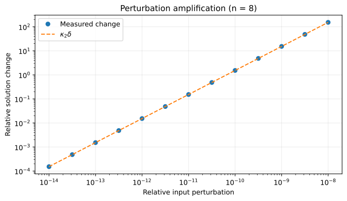
左特異ベクトル $\mathbf{u}_i$ と右特異ベクトル $\mathbf{v}_i$ は、いずれも単位ベクトルであり、$\mathbf{H}\mathbf{v}_i=\sigma_i\mathbf{u}_i$ を満たす。$\mathbf{x}=\mathbf{v}_{\max}$、$\mathbf{b}=\sigma_{\max}\mathbf{u}_{\max}$ とし、$\delta>0$ に対して $\Delta\mathbf{b}=\delta\sigma_{\max}\mathbf{u}_{\min}$ を加える。このとき、右辺の相対変化は $\delta$ であり、解の変化は次のようになる。
$$ \begin{aligned} \Delta\mathbf{x} &=\mathbf{H}^{-1}\Delta\mathbf{b} =\frac{\delta\sigma_{\max}}{\sigma_{\min}}\mathbf{v}_{\min},\\ \frac{\|\Delta\mathbf{x}\|_2}{\|\mathbf{x}\|_2} &=\delta\kappa_2(\mathbf{H}). \end{aligned} $$
このように元の解と右辺の変化方向を選ぶと、相対変化の増幅率は条件数に一致する。次のコードでは $n=8$ とし、右辺の相対変化と解の相対変化を比較する。変更前後の解はどちらも数値計算で求めるため、右辺の変化が極めて小さい場合には、丸め誤差の影響で理論値からずれることがある。
Pythonによる計算例
H = hilbert(8)
U, singular_values, Vt = np.linalg.svd(H)

# 最大特異値に対応する右特異ベクトルを元の解に選ぶ。
x_original = Vt[0]
b_original = H @ x_original
x_baseline = np.linalg.solve(H, b_original)

perturbation_sizes = np.logspace(-14, -8, 13)
relative_changes = []

for delta in perturbation_sizes:
    # 最小特異値に対応する左特異ベクトル方向へ右辺を変化させる。
    # 変化のノルムは、元の右辺のノルムのdelta倍とする。
    delta_b = delta * np.linalg.norm(b_original) * U[:, -1]
    x_shifted = np.linalg.solve(H, b_original + delta_b)

    relative_change = np.linalg.norm(x_shifted - x_baseline) / np.linalg.norm(x_baseline)
    relative_changes.append(relative_change)

condition_number = singular_values[0] / singular_values[-1]
theoretical_changes = condition_number * perturbation_sizes

# 数表でも理論値との一致を確認する。
perturbation_summary = []
for index in (0, 6, 12):
    perturbation_summary.append(
        {
            "input_change": f"{perturbation_sizes[index]:.2e}",
            "solution_change": f"{relative_changes[index]:.2e}",
            "theory": f"{theoretical_changes[index]:.2e}",
        }
    )

print("入力の相対変化と解の相対変化")
pprint(perturbation_summary, sort_dicts=False)
入力の相対変化と解の相対変化
[{'input_change': '1.00e-14',
  'solution_change': '1.52e-04',
  'theory': '1.53e-04'},
 {'input_change': '1.00e-11',
  'solution_change': '1.53e-01',
  'theory': '1.53e-01'},
 {'input_change': '1.00e-08',
  'solution_change': '1.53e+02',
  'theory': '1.53e+02'}]
# 両対数軸で、実測した変化と条件数による理論値を比較する。
fig, ax = plt.subplots(figsize=(7, 4), layout="constrained")
ax.loglog(perturbation_sizes, relative_changes, "o", label="Measured change")
ax.loglog(
    perturbation_sizes,
    theoretical_changes,
    "--",
    label=r"$\kappa_2\delta$",
)
ax.set(
    title="Perturbation amplification (n = 8)",
    xlabel="Relative input perturbation",
    ylabel="Relative solution change",
)
ax.legend()
# SVGファイルとして保存し、ノートブックにも表示する。
svg_path = figure_dir / "04_perturbation_amplification.svg"
fig.savefig(svg_path, format="svg", bbox_inches="tight")
print(f"SVG保存先: {svg_path.as_posix()}")
plt.show()
SVG保存先: figures/04_perturbation_amplification.svg
5. 精度を上げる場合の注意
数式と考え方
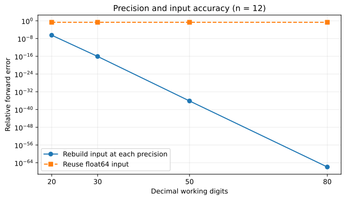
np.linalg.solve は逆行列を明示的に作らずに連立一次方程式を解くが、問題の条件数は変えない。元のHilbert行列に対する解の精度を上げるには、各成分 $1/(i+j-1)$ と右辺を多倍長精度で計算し直す必要がある。倍精度ですでに丸められた行列と右辺を多倍長に変換しても、丸めによって失われた情報は復元されない。
次の比較では $n=12$ に固定する。一方は各精度で行列と右辺を作り直し、他方は倍精度で作った入力をそのまま多倍長に変換する。どちらも、全成分が1の基準解に対する相対前進誤差を求める。後者で高精度に求められるのは、丸められた入力に対する解であり、基準解とはずれがある。
Pythonによる計算例
size = 12
H_float64 = hilbert(size)
b_float64 = H_float64 @ np.ones(size)

working_digits = [20, 30, 50, 80]
rebuilt_input_errors = []
rounded_input_errors = []

for digits in working_digits:
    with mp.workdps(digits):
        x_true = mp.matrix([1] * size)

        # 方法1: 行列と右辺を、その時点の多倍長精度で作り直す。
        H_rebuilt = make_mp_hilbert(size)
        b_rebuilt = H_rebuilt * x_true
        x_rebuilt = mp.lu_solve(H_rebuilt, b_rebuilt)

        # 方法2: 倍精度で丸められた入力を、そのまま多倍長へ変換する。
        # 計算精度を増やしても、入力時に失った情報は復元されない。
        H_rounded = mp.matrix(H_float64.tolist())
        b_rounded = mp.matrix(b_float64.tolist())
        x_rounded = mp.lu_solve(H_rounded, b_rounded)

        # 誤差も多倍長で評価し、最後に表示・描画用のfloatへ変換する。
        rebuilt_error = mp.norm(x_rebuilt - x_true) / mp.norm(x_true)
        rounded_error = mp.norm(x_rounded - x_true) / mp.norm(x_true)
        rebuilt_input_errors.append(float(rebuilt_error))
        rounded_input_errors.append(float(rounded_error))

precision_summary = []
for digits, rebuilt_error, rounded_error in zip(working_digits, rebuilt_input_errors, rounded_input_errors):
    precision_summary.append(
        {
            "digits": digits,
            "rebuilt_input_error": f"{rebuilt_error:.2e}",
            "float64_input_error": f"{rounded_error:.2e}",
        }
    )

print("入力の作り方と計算精度による相対前進誤差の比較")
pprint(precision_summary, sort_dicts=False)
入力の作り方と計算精度による相対前進誤差の比較
[{'digits': 20,
  'rebuilt_input_error': '3.15e-07',
  'float64_input_error': '2.11e-01'},
 {'digits': 30,
  'rebuilt_input_error': '8.44e-17',
  'float64_input_error': '2.11e-01'},
 {'digits': 50,
  'rebuilt_input_error': '7.19e-37',
  'float64_input_error': '2.11e-01'},
 {'digits': 80,
  'rebuilt_input_error': '1.23e-66',
  'float64_input_error': '2.11e-01'}]
# 多倍長の計算桁数と、目標の解からのずれを比較する。
fig, ax = plt.subplots(figsize=(7, 4), layout="constrained")
ax.semilogy(
    working_digits,
    rebuilt_input_errors,
    "o-",
    label="Rebuild input at each precision",
)
ax.semilogy(
    working_digits,
    rounded_input_errors,
    "s--",
    label="Reuse float64 input",
)
ax.set(
    title="Precision and input accuracy (n = 12)",
    xlabel="Decimal working digits",
    ylabel="Relative forward error",
)
ax.set_xticks(working_digits)
ax.legend()
# SVGファイルとして保存し、ノートブックにも表示する。
svg_path = figure_dir / "05_precision_and_input_accuracy.svg"
fig.savefig(svg_path, format="svg", bbox_inches="tight")
print(f"SVG保存先: {svg_path.as_posix()}")
plt.show()
SVG保存先: figures/05_precision_and_input_accuracy.svg
計算結果
80桁計算で入力を作り直した場合、基準解に対する相対前進誤差は約 $1.23\times10^{-66}$ である。倍精度で作った入力を使う場合は約 $2.11\times10^{-1}$ であり、計算桁数を増やしても基準解からのずれは残る。
結論
Hilbert行列を係数行列とする連立一次方程式では、条件数が大きいために入力や計算のわずかな誤差が増幅され、倍精度では正確な解を求めにくくなる。
逆行列が存在していても、有限精度の計算で正確な解が得られるとは限らない。残差と条件数を併せて調べ、必要なら入力を作る段階から計算精度を上げる必要がある。多項式近似でHilbert行列が現れる場合は、単項式の代わりに直交基底を使う方法も考えられる。
参考文献:NumPyの条件数の定義 。