条件数はなぜ数値計算の難しさを表すのか
※ 本記事は2015年に作成した記事のリライトになります。なお、内容は当時のものを基にしていますが、Pythonやライブラリのバージョンは最新のものを使用しています。
実行環境
Python 3.14.6(仮想環境、Jupyter Notebook)。
概要
連立一次方程式の行列を固定すると、右辺の相対誤差に対する解の相対誤差の増幅率は、行列の条件数以下になる。右辺と誤差の方向を選ぶと、この上限に達する。
本記事では、この誤差の評価式を導き、特異値と条件数の関係、誤差の方向による増幅率の違い、残差と解の誤差の違いをPythonで確認する。ここでいう「難しさ」は、入力に誤差があっても解の精度を保つ難しさである。
計算の準備
使用したライブラリのバージョンは、次の出力に示す。
import sys
from pathlib import Path
from pprint import pprint

import matplotlib
import matplotlib.pyplot as plt
import numpy as np
from IPython.display import Math, display
from matplotlib.ticker import FuncFormatter, NullFormatter
from matplotlib_inline.backend_inline import set_matplotlib_formats

%matplotlib inline

# 指定したバージョンの仮想環境で実行していることを確認する。
assert sys.version_info[:3] == (3, 14, 6)
assert sys.prefix != sys.base_prefix
print(f"実行環境: wa-src({sys.version.split()[0]})")
print(f"Python実行ファイル: {sys.executable}")
print(f"NumPy: {np.__version__}, Matplotlib: {matplotlib.__version__}")

# 配列の数値とグラフの目盛を、表示時だけ有効数字3桁に整える。
np.set_printoptions(formatter={"float_kind": lambda value: f"{value:.2e}"})
tick_formatter = FuncFormatter(lambda value, position: f"{value:#.3g}")
set_matplotlib_formats("svg")
plt.rcParams.update({
    "figure.figsize": (7, 4),
    "font.size": 10,
    "axes.grid": True,
    "grid.alpha": 0.250,
    "savefig.format": "svg",
    "svg.fonttype": "none",
})
figure_dir = Path("figures")
figure_dir.mkdir(parents=True, exist_ok=True)


def latex_number(value):
    """数値を有効数字3桁のLaTeX表記に変換する。"""
    mantissa, exponent = f"{float(value):.2e}".split("e")
    return rf"{mantissa}\times 10^{{{int(exponent)}}}"


def save_figure(fig, filename):
    """目盛の表記を整え、SVG保存とノートブック表示を行う。"""
    for ax in fig.axes:
        for axis in (ax.xaxis, ax.yaxis):
            if axis.get_scale() == "linear":
                axis.set_major_formatter(tick_formatter)
            # 対数軸は整数の指数で表示し、補助目盛の数値を隠す。
            axis.set_minor_formatter(NullFormatter())
    output_path = figure_dir / filename
    fig.savefig(output_path, format="svg", bbox_inches="tight")
    print(f"SVG保存先: {output_path.as_posix()}")
    plt.show()
実行環境: wa-src(3.14.6)
Python実行ファイル: /Users/hiroshi/private/wa_src/.venv/bin/python
NumPy: 2.5.4, Matplotlib: 3.11.2
1. 相対誤差から条件数を導く
実数を成分とする正則な正方行列を $\mathbf{A}$ とし、$\mathbf{A}\mathbf{x}=\mathbf{b}$、$\mathbf{b}\ne\mathbf{0}$ とする。以下では、ベクトルのユークリッドノルムと、それに対応する行列の2ノルムを使う。
$$ \begin{aligned} \|\mathbf{v}\|_2&=\sqrt{\sum_i v_i^2},\\ \|\mathbf{A}\|_2&=\max_{\mathbf{v}\ne\mathbf{0}} \frac{\|\mathbf{A}\mathbf{v}\|_2}{\|\mathbf{v}\|_2}. \end{aligned} $$
まず行列を固定し、右辺に変化 $\Delta\mathbf{b}$ を加える。変化後の解を $\mathbf{x}+\Delta\mathbf{x}$ とおくと、次の関係が成り立つ。
$$ \begin{aligned} \mathbf{A}(\mathbf{x}+\Delta\mathbf{x})&=\mathbf{b}+\Delta\mathbf{b},\\ \mathbf{A}\mathbf{x}+\mathbf{A}\Delta\mathbf{x}&=\mathbf{b}+\Delta\mathbf{b},\\ \mathbf{A}\Delta\mathbf{x}&=\Delta\mathbf{b},\\ \Delta\mathbf{x}&=\mathbf{A}^{-1}\Delta\mathbf{b},\\ \|\Delta\mathbf{x}\|_2&\le\|\mathbf{A}^{-1}\|_2\|\Delta\mathbf{b}\|_2. \end{aligned} $$
また、$\|\mathbf{b}\|_2=\|\mathbf{A}\mathbf{x}\|_2\le\|\mathbf{A}\|_2\|\mathbf{x}\|_2$ が成り立つ。これを使うと、相対誤差を次のように評価できる。
$$ \begin{aligned} \frac{\|\Delta\mathbf{x}\|_2}{\|\mathbf{x}\|_2} &\le\frac{\|\mathbf{A}^{-1}\|_2\|\Delta\mathbf{b}\|_2}{\|\mathbf{x}\|_2}\\ &\le\|\mathbf{A}^{-1}\|_2\|\mathbf{A}\|_2 \frac{\|\Delta\mathbf{b}\|_2}{\|\mathbf{b}\|_2}. \end{aligned} $$
この不等式に現れる $\|\mathbf{A}^{-1}\|_2\|\mathbf{A}\|_2$ が、2ノルムに基づく行列の条件数である。
$$ \boxed{\kappa_2(\mathbf{A})=\|\mathbf{A}\|_2\|\mathbf{A}^{-1}\|_2}. $$
$$ \frac{\|\Delta\mathbf{x}\|_2}{\|\mathbf{x}\|_2} \le\kappa_2(\mathbf{A})\frac{\|\Delta\mathbf{b}\|_2}{\|\mathbf{b}\|_2}. $$
行列を固定して右辺だけを変える場合、この評価は変化が微小でなくても成り立つ。条件数は、右辺 $\mathbf{b}$ と誤差 $\Delta\mathbf{b}$ の方向を選んだときに得られる最大の増幅率である。この評価は Driscoll・Braunの教科書 でも示されている。
2. 特異値と図形の変形
特異値分解を $\mathbf{A}=\mathbf{U}\mathbf{\Sigma}\mathbf{V}^{\mathsf T}$ とする。$\mathbf{U},\mathbf{V}$ は直交行列であり、ベクトルの長さを変えない。$\mathbf{\Sigma}$ は、正の特異値を対角成分に持つ対角行列である。特異値の最大値を $\sigma_{\max}$、最小値を $\sigma_{\min}$ とすると、次の関係が成り立つ。
$$ \begin{aligned} \|\mathbf{A}\|_2&=\sigma_{\max},\\ \mathbf{A}^{-1}&=\mathbf{V}\mathbf{\Sigma}^{-1}\mathbf{U}^{\mathsf T},\\ \|\mathbf{A}^{-1}\|_2&=\max_i\frac{1}{\sigma_i}=\frac{1}{\sigma_{\min}},\\ \kappa_2(\mathbf{A})&=\frac{\sigma_{\max}}{\sigma_{\min}}\ge1. \end{aligned} $$
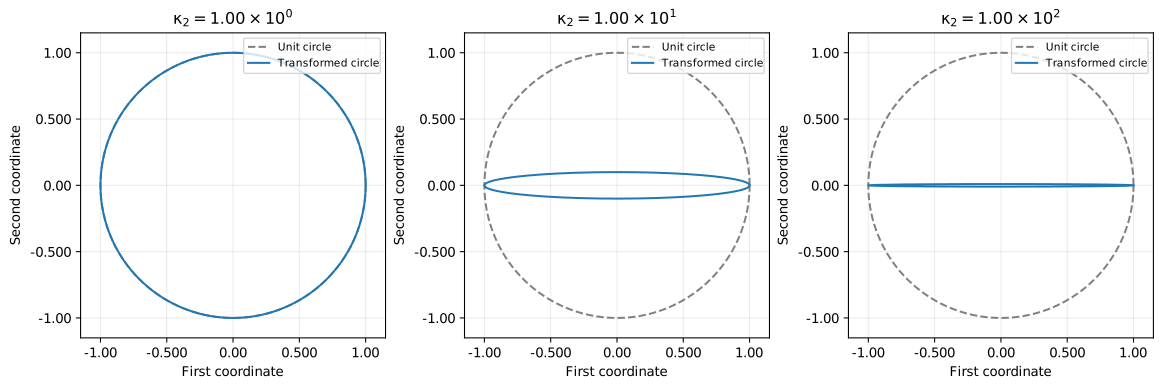
2次元では、行列 $\mathbf{A}$ によって単位円が楕円に変換される。その長半径と短半径は、それぞれ $\sigma_{\max}$ と $\sigma_{\min}$ である。楕円を単位円に戻すとき、逆行列 $\mathbf{A}^{-1}$ は短軸方向のベクトルの長さを $1/\sigma_{\min}$ 倍にする。条件数は、この長半径と短半径の比に等しい。なお、特異行列の条件数は無限大と定義する。
Pythonによる計算例
np.linalg.cond は、デフォルトでは特異値分解を用いて2ノルムの条件数を計算する(NumPyの公式ドキュメント
)。
# 対角行列では特異値が対角成分の絶対値になる。
A = np.diag([1, 0.0100])
singular_values = np.linalg.svd(A, compute_uv=False)
kappa = np.linalg.cond(A)
print("特異値(降順)")
pprint(singular_values)
display(Math(
    rf"\kappa_2(\mathbf{{A}})="
    rf"\frac{{{latex_number(singular_values[0])}}}"
    rf"{{{latex_number(singular_values[-1])}}}={latex_number(kappa)}"
))

# 同じ単位円を、異なる条件数の行列で変換する。
theta = np.linspace(0, 2 * np.pi, 721)
unit_circle = np.vstack([np.cos(theta), np.sin(theta)])
fig, axes = plt.subplots(1, 3, figsize=(12, 4), layout="constrained")
for ax, alpha in zip(axes, [1, 0.100, 0.0100]):
    matrix = np.diag([1, alpha])
    ellipse = matrix @ unit_circle
    ax.plot(*unit_circle, "--", color="gray", label="Unit circle")
    ax.plot(*ellipse, color="tab:blue", label="Transformed circle")
    ax.set(
        xlabel="First coordinate", ylabel="Second coordinate",
        xlim=(-1.15, 1.15), ylim=(-1.15, 1.15),
        title=rf"$\kappa_2={latex_number(np.linalg.cond(matrix))}$",
    )
    ax.set_aspect("equal")
    ax.legend(loc="upper right", fontsize=8)
save_figure(fig, "01_circle_and_ellipses.svg")
特異値(降順)
array([1.00e+00, 1.00e-02])
$$ \displaystyle \kappa_2(\mathbf{A})=\frac{1.00\times 10^{0}}{1.00\times 10^{-2}}=1.00\times 10^{2} $$
SVG保存先: figures/01_circle_and_ellipses.svg
3. 相対誤差が条件数倍になる例
$0<\alpha\le1$、$\eta>0$ として次の問題を考える。
$$ \mathbf{A}=\begin{bmatrix}1&0\\0&\alpha\end{bmatrix},\quad \mathbf{b}=\begin{bmatrix}1\\0\end{bmatrix},\quad \Delta\mathbf{b}=\begin{bmatrix}0\\\eta\end{bmatrix}. $$
第1式と第2式は、それぞれ $x_1=1$ と $\alpha x_2=0$ である。変化後の第2式は $\alpha(x_2+\Delta x_2)=\eta$ となる。したがって、解の変化と相対誤差は次のように求められる。
$$ \mathbf{x}=\begin{bmatrix}1\\0\end{bmatrix},\quad \Delta\mathbf{x}=\begin{bmatrix}0\\\eta/\alpha\end{bmatrix}. $$
$$ \frac{\|\Delta\mathbf{x}\|_2}{\|\mathbf{x}\|_2} =\frac{\eta}{\alpha}=\kappa_2(\mathbf{A})\eta. $$
$\alpha=1.00\times10^{-3}$、$\eta=1.00\times10^{-6}$ なら、入力の相対誤差は $1.00\times10^{-6}$、解の相対誤差は $1.00\times10^{-3}$ になる。以下では、右辺に意図的な誤差を加え、相対誤差の増幅率を確かめる。逆行列は式の導出に用い、解の計算には np.linalg.solve を使う。
alpha = 1.00e-3
eta = 1.00e-6
A = np.diag([1, alpha])
b = np.array([1, 0], dtype=float)
delta_b = np.array([0, eta])
x = np.linalg.solve(A, b)
x_changed = np.linalg.solve(A, b + delta_b)
input_error = np.linalg.norm(delta_b) / np.linalg.norm(b)
solution_error = np.linalg.norm(x_changed - x) / np.linalg.norm(x)

print("元の解と変化後の解(行ごと)")
pprint(np.vstack([x, x_changed]))
# 辞書内の数値も有効数字3桁に整えてpprintで表示する。
pprint({
    "input_relative_error": f"{input_error:.2e}",
    "solution_relative_error": f"{solution_error:.2e}",
    "amplification": f"{solution_error / input_error:.2e}",
})
display(Math(
    rf"\kappa_2(\mathbf{{A}})\eta="
    rf"{latex_number(np.linalg.cond(A) * input_error)}"
))
元の解と変化後の解(行ごと)
array([[1.00e+00, 0.00e+00],
       [1.00e+00, 1.00e-03]])
{'amplification': '1.00e+03',
 'input_relative_error': '1.00e-06',
 'solution_relative_error': '1.00e-03'}
$$ \displaystyle \kappa_2(\mathbf{A})\eta=1.00\times 10^{-3} $$
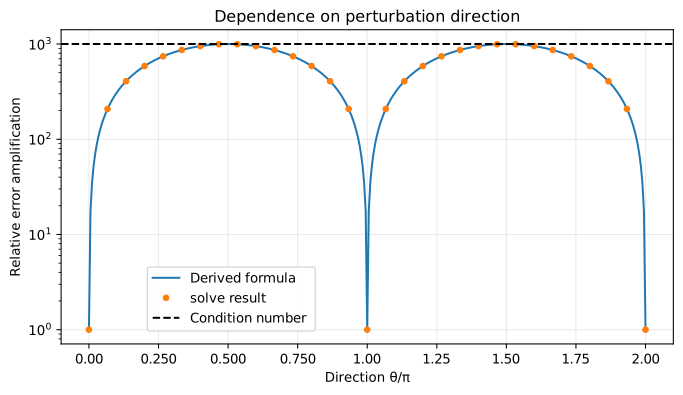
次に、誤差の大きさを固定して方向だけを変える。誤差を $\Delta\mathbf{b}=\eta(\cos\theta,\sin\theta)^{\mathsf T}$ とすると、解の変化は $\eta(\cos\theta,\sin\theta/\alpha)^{\mathsf T}$ である。相対誤差の増幅率は次のようになる。
$$ \frac{\|\Delta\mathbf{x}\|_2/\|\mathbf{x}\|_2} {\|\Delta\mathbf{b}\|_2/\|\mathbf{b}\|_2} =\sqrt{\cos^2\theta+\frac{\sin^2\theta}{\alpha^2}}. $$
$\theta=0$ では 1 倍、$\theta=\pi/2$ では $1/\alpha$ 倍となる。同じ大きさの誤差でも、方向によって増幅率が異なる。
# 同じ大きさの入力誤差を回転させ、増幅率を比較する。
angles = np.linspace(0, 2 * np.pi, 361)
amplifications = []
for angle in angles:
    perturbation = eta * np.array([np.cos(angle), np.sin(angle)])
    perturbed_x = np.linalg.solve(A, b + perturbation)
    relative_change = np.linalg.norm(perturbed_x - x) / np.linalg.norm(x)
    amplifications.append(relative_change / eta)

direction_formula = np.sqrt(np.cos(angles)**2 + np.sin(angles)**2 / alpha**2)
fig, ax = plt.subplots(layout="constrained")
ax.semilogy(angles / np.pi, direction_formula, label="Derived formula")
ax.semilogy(
    angles[::12] / np.pi, np.array(amplifications)[::12],
    "o", markersize=4, label="solve result",
)
ax.axhline(np.linalg.cond(A), color="black", linestyle="--", label="Condition number")
ax.set(xlabel=r"Direction $\theta/\pi$", ylabel="Relative error amplification",
       title="Dependence on perturbation direction")
ax.legend(loc="lower left", bbox_to_anchor=(0.130, 0.0200))
save_figure(fig, "02_direction_and_amplification.svg")
SVG保存先: figures/02_direction_and_amplification.svg
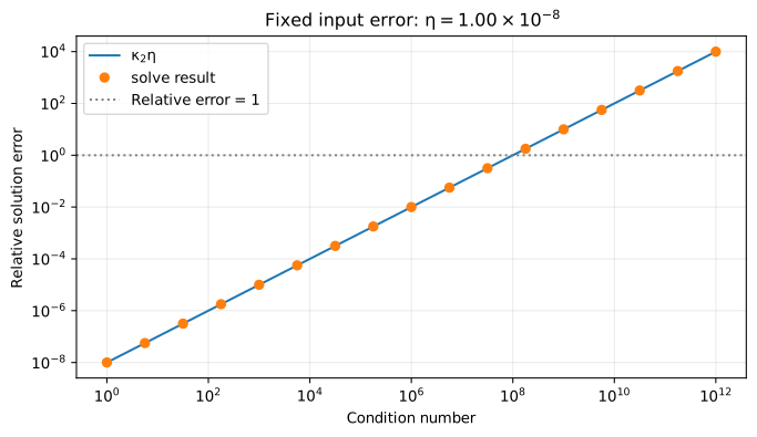
続いて、右辺の相対誤差を $\eta=1.00\times10^{-8}$ に固定し、最も増幅される方向に誤差を加える。$\alpha$ を変えて条件数を大きくすると、解の相対誤差が条件数に比例して大きくなることを確かめる。
# 入力誤差を固定し、最も増幅される方向で条件数との関係を調べる。
eta_sweep = 1.00e-8
alphas = np.logspace(0, -12, 49)
condition_numbers = []
relative_errors = []
for alpha_value in alphas:
    matrix = np.diag([1, alpha_value])
    changed = np.linalg.solve(matrix, b + np.array([0, eta_sweep]))
    condition_numbers.append(np.linalg.cond(matrix))
    relative_errors.append(np.linalg.norm(changed - x) / np.linalg.norm(x))
condition_numbers = np.array(condition_numbers)
relative_errors = np.array(relative_errors)

print("各行: 条件数、入力相対誤差、解の相対誤差")
pprint(np.column_stack([
    condition_numbers[::16], np.full(4, eta_sweep), relative_errors[::16],
]))
fig, ax = plt.subplots(layout="constrained")
ax.loglog(condition_numbers, condition_numbers * eta_sweep, label=r"$\kappa_2\eta$")
ax.loglog(condition_numbers[::3], relative_errors[::3], "o", label="solve result")
ax.axhline(1, color="gray", linestyle=":", label="Relative error = 1")
ax.set(xlabel="Condition number", ylabel="Relative solution error",
       title="Fixed input error: " + rf"$\eta={latex_number(eta_sweep)}$")
ax.legend()
save_figure(fig, "03_condition_number_and_error.svg")
各行: 条件数、入力相対誤差、解の相対誤差
array([[1.00e+00, 1.00e-08, 1.00e-08],
       [1.00e+04, 1.00e-08, 1.00e-04],
       [1.00e+08, 1.00e-08, 1.00e+00],
       [1.00e+12, 1.00e-08, 1.00e+04]])


SVG保存先: figures/03_condition_number_and_error.svg
4. 行列式の大きさだけでは判断できない
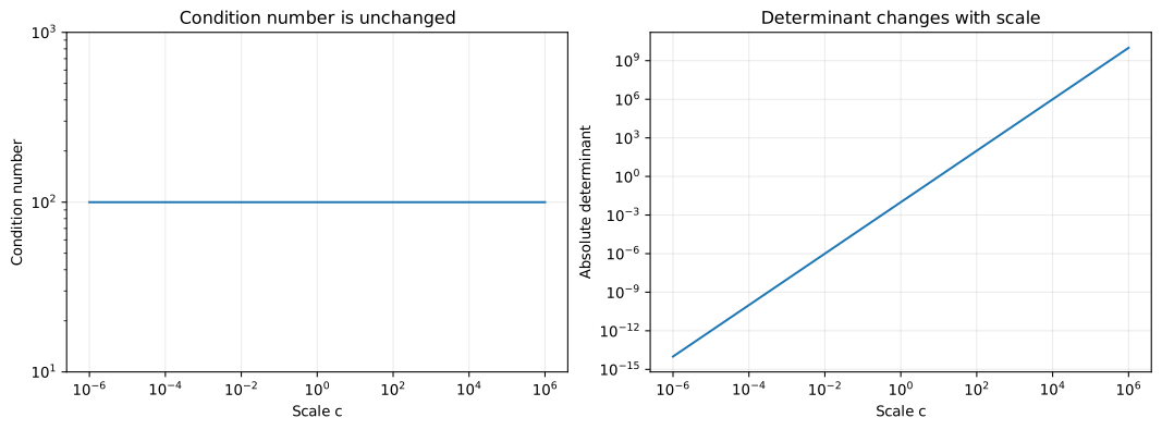
行列 $\mathbf{A}$ 全体をゼロでない定数 $c$ 倍しても、条件数は変わらない。一方、$n$ 次正方行列の行列式は $c^n$ 倍になる。
$$ \begin{aligned} \kappa_2(c\mathbf{A}) &=\|c\mathbf{A}\|_2\|(c\mathbf{A})^{-1}\|_2\\ &=|c|\|\mathbf{A}\|_2\frac{1}{|c|}\|\mathbf{A}^{-1}\|_2 =\kappa_2(\mathbf{A}),\\ \det(c\mathbf{A})&=c^n\det(\mathbf{A}). \end{aligned} $$
したがって、行列式の絶対値が小さいという理由だけで、入力誤差が増幅されやすいとは判断できない。次の図では、同じ行列を定数倍したときの条件数と行列式の絶対値を比較する。
base_matrix = np.diag([1, 0.0100])
scales = np.logspace(-6, 6, 49)
scaled_conditions = np.array([np.linalg.cond(c * base_matrix) for c in scales])
scaled_determinants = np.array([abs(np.linalg.det(c * base_matrix)) for c in scales])

fig, axes = plt.subplots(1, 2, figsize=(11, 4), layout="constrained")
# 定数系列の自動範囲計算を避けるため、描画前に縦軸の範囲を指定する。
axes[0].set(xscale="log", yscale="log", ylim=(10, 1000))
axes[0].plot(scales, scaled_conditions)
axes[0].set(xlabel="Scale c", ylabel="Condition number",
            title="Condition number is unchanged")
axes[1].loglog(scales, scaled_determinants)
axes[1].set(xlabel="Scale c", ylabel="Absolute determinant",
            title="Determinant changes with scale")
save_figure(fig, "04_scaling_and_determinant.svg")
SVG保存先: figures/04_scaling_and_determinant.svg
5. 残差と計算方法の安定性
近似解を $\widehat{\mathbf{x}}$ とし、残差を $\mathbf{r}=\mathbf{b}-\mathbf{A}\widehat{\mathbf{x}}$ と定義する。
$$ \begin{aligned} \mathbf{r}&=\mathbf{A}\mathbf{x}-\mathbf{A}\widehat{\mathbf{x}} =\mathbf{A}(\mathbf{x}-\widehat{\mathbf{x}}),\\ \mathbf{x}-\widehat{\mathbf{x}}&=\mathbf{A}^{-1}\mathbf{r},\\ \frac{\|\mathbf{x}-\widehat{\mathbf{x}}\|_2}{\|\mathbf{x}\|_2} &\le\kappa_2(\mathbf{A})\frac{\|\mathbf{r}\|_2}{\|\mathbf{b}\|_2}. \end{aligned} $$
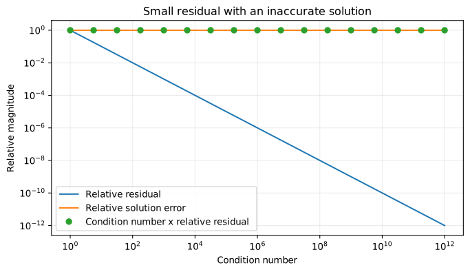
第3節と同じ行列 $\mathbf{A}$ と右辺 $\mathbf{b}$ を用い、近似解を意図的に $\widehat{\mathbf{x}}=(1,1)^{\mathsf T}$ とおく。このとき残差は $\mathbf{r}=(0,-\alpha)^{\mathsf T}$ となる。相対残差は $\alpha$ だが、解の相対誤差は1である。$\alpha$ を小さくすれば相対残差はいくらでも小さくなるが、解の相対誤差は変わらない。このように、残差が小さいだけでは解の精度を保証できない。
# solveの出力ではなく、残差と誤差の違いを示すために作った近似解である。
x_hat = np.array([1, 1], dtype=float)
relative_residuals = []
forward_errors = []
for alpha_value in alphas:
    matrix = np.diag([1, alpha_value])
    residual = b - matrix @ x_hat
    relative_residuals.append(np.linalg.norm(residual) / np.linalg.norm(b))
    forward_errors.append(np.linalg.norm(x_hat - x) / np.linalg.norm(x))
relative_residuals = np.array(relative_residuals)
forward_errors = np.array(forward_errors)

print("各行: 条件数、相対残差、解の相対誤差")
pprint(np.column_stack([
    condition_numbers[::16], relative_residuals[::16], forward_errors[::16],
]))
fig, ax = plt.subplots(layout="constrained")
ax.loglog(condition_numbers, relative_residuals, label="Relative residual")
ax.loglog(condition_numbers, forward_errors, label="Relative solution error")
ax.loglog(
    condition_numbers[::3], (condition_numbers * relative_residuals)[::3],
    "o", label="Condition number x relative residual",
)
ax.set(xlabel="Condition number", ylabel="Relative magnitude",
       title="Small residual with an inaccurate solution")
ax.legend()
save_figure(fig, "05_residual_and_solution_error.svg")
各行: 条件数、相対残差、解の相対誤差
array([[1.00e+00, 1.00e+00, 1.00e+00],
       [1.00e+04, 1.00e-04, 1.00e+00],
       [1.00e+08, 1.00e-08, 1.00e+00],
       [1.00e+12, 1.00e-12, 1.00e+00]])
SVG保存先: figures/05_residual_and_solution_error.svg
関係式 $\mathbf{A}\widehat{\mathbf{x}}=\mathbf{b}-\mathbf{r}$ は、右辺を $-\mathbf{r}$ だけ変えれば、近似解 $\widehat{\mathbf{x}}$ がその方程式の厳密解になることを示している。したがって、相対残差は、行列を固定して右辺だけを変える場合の相対後退誤差である。一方、近似解と元の方程式の厳密解との差を測るのが前進誤差であり、ここでは解の相対誤差として評価している。
後退安定な計算方法は、入力に丸め誤差程度の小さな変更を加えた問題の厳密解を返す。しかし、条件数が大きい問題では、入力のわずかな変化が解の大きな変化につながることがある。条件数は問題の性質であり、安定性は計算方法の性質である。
右辺の相対誤差を $10^{-p}$、条件数を $10^q$ とすると、解の相対誤差の上限は $10^{q-p}$ となる。$p>q$ なら、最悪の場合に有効数字が約 $q$ 桁失われると考えられる。$p\le q$ では上限が1以上となり、この評価からは有効桁を保証できない。ただし、実際に失われる桁数は、右辺や誤差の方向によって変わる。測定による入力誤差は、計算の桁数を増やすだけでは取り除けない。
結論
行列を固定して右辺に誤差を加えると、解の相対誤差は、右辺の相対誤差に条件数を掛けた値以下になる。右辺と誤差の方向を選べば、この上限に達する場合がある。
2ノルムの条件数は最大特異値と最小特異値の比であり、実際の増幅率は右辺や誤差の方向によって変わる。解の精度を判断するには、残差の小ささに加え、条件数、入力の精度、計算方法の安定性を確かめる必要がある。